机器学习：SVM（非线性数据分类：SVM中使用多项式特征和核函数SVC）

一、基础理解

数据：线性数据、非线性数据；
线性数据：线性相关、非线性相关；（非线性相关的数据不一定是非线性数据）

　1）SVM 解决非线性数据分类的方法

方法一：
多项式思维：扩充原本的数据，制造新的多项式特征；（对每一个样本添加多项式特征）
步骤：

PolynomialFeatures(degree = degree)：扩充原始数据，生成多项式特征；
StandardScaler()：标准化处理扩充后的数据；
LinearSVC(C = C)：使用 SVM 算法训练模型；

方法二：
使用scikit-learn 中封装好的核函数： SVC(kernel='poly', degree=degree, C=C)
功能：当 SVC() 的参数 kernel = ‘poly’ 时，直接使用多项式特征处理数据；

注：使用 SVC() 前，也需要对数据进行标准化处理

二、例

　1）生成数据

datasets.make_ + 后缀：自动生成数据集；

如果想修改生成的数据量，可在make_moons()中填入参数；

import numpy as np

import matplotlib.pyplot as plt

from sklearn import datasets

X, y = datasets.make_moons(noise=0.15, random_state=666)

plt.scatter(X[y==0, 0], X[y==0, 1])

plt.scatter(X[y==1, 0], X[y==1, 1])

plt.show()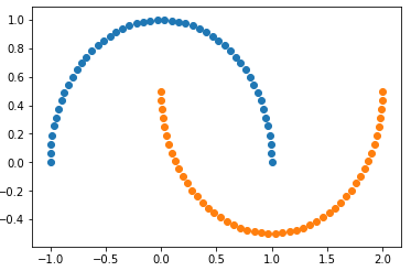

　2）绘图函数

def plot_decision_boundary(model, axis):

    x0, x1 = np.meshgrid(

        np.linspace(axis[0], axis[1], int((axis[1]-axis[0])*100)).reshape(-1,1),

        np.linspace(axis[2], axis[3], int((axis[3]-axis[2])*100)).reshape(-1,1)

    )

    X_new = np.c_[x0.ravel(), x1.ravel()]

    y_predict = model.predict(X_new)

    zz = y_predict.reshape(x0.shape)

    from matplotlib.colors import ListedColormap

    custom_cmap = ListedColormap(['#EF9A9A','#FFF59D','#90CAF9'])

    plt.contourf(x0, x1, zz, linewidth=5, cmap=custom_cmap)

　3）方法一：多项式思维

from sklearn.preprocessing import PolynomialFeatures, StandardScaler

from sklearn.svm import LinearSVC

from sklearn.pipeline import Pipeline

def PolynomialSVC(degree, C=1.0):

    return Pipeline([

        ('poly', PolynomialFeatures(degree=degree)),

        ('std)scaler', StandardScaler()),

        ('linearSVC', LinearSVC(C=C))

    ])

poly_svc = PolynomialSVC(degree=3)

poly_svc.fit(X, y)

plot_decision_boundary(poly_svc, axis=[-1.5, 2.5, -1.0, 1.5])

plt.scatter(X[y==0, 0], X[y==0, 1])

plt.scatter(X[y==1, 0], X[y==1, 1])

plt.show()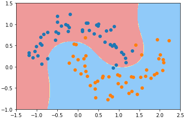

改变参数：degree、C，模型的决策边界也跟着改变；

　4）方法二：使用核函数 SVC()

对于SVM算法，在scikit-learn的封装中，可以不使用 PolynomialFeatures的方式先将数据转化为高维的具有多项式特征的数据，在将数据提供给算法;

SVC() 算法：直接使用多项式特征；

from sklearn.svm import SVC

# 当算法SVC()的参数 kernel='poly'时，SVC()能直接打到一种多项式特征的效果；

# 使用 SVC() 前，也需要对数据进行标准化处理

def PolynomialKernelSVC(degree, C=1.0):

    return Pipeline([

        ('std_scaler', StandardScaler()),

        ('kernelSVC', SVC(kernel='poly', degree=degree, C=C))

    ])

poly_kernel_svc = PolynomialKernelSVC(degree=3)

poly_kernel_svc.fit(X, y)

plot_decision_boundary(poly_kernel_svc, axis=[-1.5, 2.5, -1.0, 1.5])

plt.scatter(X[y==0, 0], X[y==0, 1])

plt.scatter(X[y==1, 0], X[y==1, 1])

plt.show()

调整 PolynomialkernelSVC() 的参数：degree、C，可改决策边界；

巴特西

机器学习：SVM（非线性数据分类：SVM中使用多项式特征和核函数SVC）

一、基础理解

1）SVM 解决非线性数据分类的方法

方法一：

方法二：

二、例

1）生成数据

2）绘图函数

3）方法一：多项式思维

4）方法二：使用核函数 SVC()

最新文章

热门文章