吴裕雄--天生自然python机器学习：支持向量机SVM

基于最大间隔分隔数据

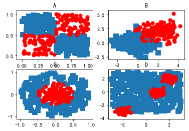
import matplotlib

import matplotlib.pyplot as plt

from numpy import *

xcord0 = []

ycord0 = []

xcord1 = []

ycord1 = []

markers =[]

colors =[]

fr = open('F:\\machinelearninginaction\\Ch06\\testSet.txt')#this file was generated by 2normalGen.py

for line in fr.readlines():

    lineSplit = line.strip().split('\t')

    xPt = float(lineSplit[0])

    yPt = float(lineSplit[1])

    label = int(lineSplit[2])

    if (label == 0):

        xcord0.append(xPt)

        ycord0.append(yPt)

    else:

        xcord1.append(xPt)

        ycord1.append(yPt)

fr.close()

fig = plt.figure()

ax = fig.add_subplot(221)

xcord0 = []; ycord0 = []; xcord1 = []; ycord1 = []

for i in range(300):

    [x,y] = random.uniform(0,1,2)

    if ((x > 0.5) and (y < 0.5)) or ((x < 0.5) and (y > 0.5)):

        xcord0.append(x); ycord0.append(y)

    else:

        xcord1.append(x); ycord1.append(y)

ax.scatter(xcord0,ycord0, marker='s', s=90)

ax.scatter(xcord1,ycord1, marker='o', s=50, c='red')

plt.title('A')

ax = fig.add_subplot(222)

xcord0 = random.standard_normal(150); ycord0 = random.standard_normal(150)

xcord1 = random.standard_normal(150)+2.0; ycord1 = random.standard_normal(150)+2.0

ax.scatter(xcord0,ycord0, marker='s', s=90)

ax.scatter(xcord1,ycord1, marker='o', s=50, c='red')

plt.title('B')

ax = fig.add_subplot(223)

xcord0 = []

ycord0 = []

xcord1 = []

ycord1 = []

for i in range(300):

    [x,y] = random.uniform(0,1,2)

    if (x > 0.5):

        xcord0.append(x*cos(2.0*pi*y)); ycord0.append(x*sin(2.0*pi*y))

    else:

        xcord1.append(x*cos(2.0*pi*y)); ycord1.append(x*sin(2.0*pi*y))

ax.scatter(xcord0,ycord0, marker='s', s=90)

ax.scatter(xcord1,ycord1, marker='o', s=50, c='red')

plt.title('C')

ax = fig.add_subplot(224)

xcord1 = zeros(150); ycord1 = zeros(150)

xcord0 = random.uniform(-3,3,350); ycord0 = random.uniform(-3,3,350);

xcord1[0:50] = 0.3*random.standard_normal(50)+2.0; ycord1[0:50] = 0.3*random.standard_normal(50)+2.0

xcord1[50:100] = 0.3*random.standard_normal(50)-2.0; ycord1[50:100] = 0.3*random.standard_normal(50)-3.0

xcord1[100:150] = 0.3*random.standard_normal(50)+1.0; ycord1[100:150] = 0.3*random.standard_normal(50)

ax.scatter(xcord0,ycord0, marker='s', s=90)

ax.scatter(xcord1,ycord1, marker='o', s=50, c='red')

plt.title('D')

plt.show()

寻找最大间隔

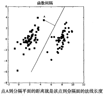
分类器求解的优化问题

这里的类别标签为什么采用-1和+1，而不是0和 1呢？这是由于-1和+1仅仅相差一个符号，
方便数学上的处理。我们可以通过一个统一公式来表示间隔或者数据点到分隔超平面的距离，同
时不必担心数据到底是属于-1还是+1类。

S V M 应用的一般框架

from numpy import *

from time import sleep

def loadDataSet(fileName):

    dataMat = []; labelMat = []

    fr = open(fileName)

    for line in fr.readlines():

        lineArr = line.strip().split('\t')

        dataMat.append([float(lineArr[0]), float(lineArr[1])])

        labelMat.append(float(lineArr[2]))

    return dataMat,labelMat

def selectJrand(i,m):

    j=i #we want to select any J not equal to i

    while (j==i):

        j = int(random.uniform(0,m))

    return j

def clipAlpha(aj,H,L):

    if aj > H:

        aj = H

    if L > aj:

        aj = L

    return aj

dataMat,labelMat = loadDataSet('F:\\machinelearninginaction\\Ch06\\testSet.txt')

print(labelMat)

可以看得出来，这里采用的类别标签是-1和1

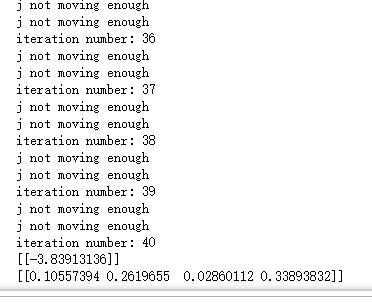
def smoSimple(dataMatIn, classLabels, C, toler, maxIter):

    dataMatrix = mat(dataMatIn); labelMat = mat(classLabels).transpose()

    b = 0; m,n = shape(dataMatrix)

    alphas = mat(zeros((m,1)))

    iter = 0

    while (iter < maxIter):

        alphaPairsChanged = 0

        for i in range(m):

            fXi = float(multiply(alphas,labelMat).T*(dataMatrix*dataMatrix[i,:].T)) + b

            Ei = fXi - float(labelMat[i])#if checks if an example violates KKT conditions

            if ((labelMat[i]*Ei < -toler) and (alphas[i] < C)) or ((labelMat[i]*Ei > toler) and (alphas[i] > 0)):

                j = selectJrand(i,m)

                fXj = float(multiply(alphas,labelMat).T*(dataMatrix*dataMatrix[j,:].T)) + b

                Ej = fXj - float(labelMat[j])

                alphaIold = alphas[i].copy()

                alphaJold = alphas[j].copy()

                if (labelMat[i] != labelMat[j]):

                    L = max(0, alphas[j] - alphas[i])

                    H = min(C, C + alphas[j] - alphas[i])

                else:

                    L = max(0, alphas[j] + alphas[i] - C)

                    H = min(C, alphas[j] + alphas[i])

                if L==H:

                    print("L==H")

                    continue

                eta = 2.0 * dataMatrix[i,:]*dataMatrix[j,:].T - dataMatrix[i,:]*dataMatrix[i,:].T - dataMatrix[j,:]*dataMatrix[j,:].T

                if eta >= 0:

                    print("eta>=0")

                    continue

                alphas[j] -= labelMat[j]*(Ei - Ej)/eta

                alphas[j] = clipAlpha(alphas[j],H,L)

                if (abs(alphas[j] - alphaJold) < 0.00001):

                    print("j not moving enough")

                    continue

                alphas[i] += labelMat[j]*labelMat[i]*(alphaJold - alphas[j])#update i by the same amount as j

                                                                        #the update is in the oppostie direction

                b1 = b - Ei- labelMat[i]*(alphas[i]-alphaIold)*dataMatrix[i,:]*dataMatrix[i,:].T - labelMat[j]*(alphas[j]-alphaJold)*dataMatrix[i,:]*dataMatrix[j,:].T

                b2 = b - Ej- labelMat[i]*(alphas[i]-alphaIold)*dataMatrix[i,:]*dataMatrix[j,:].T - labelMat[j]*(alphas[j]-alphaJold)*dataMatrix[j,:]*dataMatrix[j,:].T

                if (0 < alphas[i]) and (C > alphas[i]):

                    b = b1

                elif (0 < alphas[j]) and (C > alphas[j]):

                    b = b2

                else:

                    b = (b1 + b2)/2.0

                alphaPairsChanged += 1

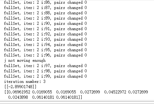
                print("iter: %d i:%d, pairs changed %d" % (iter,i,alphaPairsChanged))

        if (alphaPairsChanged == 0): iter += 1

        else: iter = 0

        print("iteration number: %d" % iter)

    return b,alphas

该函数有5个输人参数，分别
是：数据集、类别标签、常数C 、容错率和取消前最大的循环次数。

b,alphas = smoSimple(dataMat,labelMat, 0.6, 0.001, 40)

print(b)

print(alphas[alphas>0])

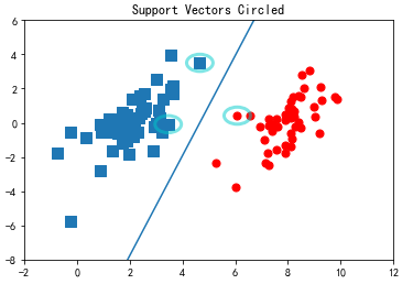
在原始数据集上对这些支持向量画圈之后的结果

import matplotlib

import matplotlib.pyplot as plt

from numpy import *

from matplotlib.patches import Circle

xcord0 = []

ycord0 = []

xcord1 = []

ycord1 = []

markers =[]

colors =[]

fr = open('F:\\machinelearninginaction\\Ch06\\testSet.txt')#this file was generated by 2normalGen.py

for line in fr.readlines():

    lineSplit = line.strip().split('\t')

    xPt = float(lineSplit[0])

    yPt = float(lineSplit[1])

    label = int(lineSplit[2])

    if (label == -1):

        xcord0.append(xPt)

        ycord0.append(yPt)

    else:

        xcord1.append(xPt)

        ycord1.append(yPt)

fr.close()

fig = plt.figure()

ax = fig.add_subplot(111)

ax.scatter(xcord0,ycord0, marker='s', s=90)

ax.scatter(xcord1,ycord1, marker='o', s=50, c='red')

plt.title('Support Vectors Circled')

circle = Circle((4.6581910000000004, 3.507396), 0.5, facecolor='none', edgecolor=(0,0.8,0.8), linewidth=3, alpha=0.5)

ax.add_patch(circle)

circle = Circle((3.4570959999999999, -0.082215999999999997), 0.5, facecolor='none', edgecolor=(0,0.8,0.8), linewidth=3, alpha=0.5)

ax.add_patch(circle)

circle = Circle((6.0805730000000002, 0.41888599999999998), 0.5, facecolor='none', edgecolor=(0,0.8,0.8), linewidth=3, alpha=0.5)

ax.add_patch(circle)

#plt.plot([2.3,8.5], [-6,6]) #seperating hyperplane

b = -3.75567

w0=0.8065

w1=-0.2761

x = arange(-2.0, 12.0, 0.1)

y = (-w0*x - b)/w1

ax.plot(x,y)

ax.axis([-2,12,-8,6])

plt.show()

def kernelTrans(X, A, kTup): #calc the kernel or transform data to a higher dimensional space

    m,n = shape(X)

    K = mat(zeros((m,1)))

    if kTup[0]=='lin':

        K = X * A.T   #linear kernel

    elif kTup[0]=='rbf':

        for j in range(m):

            deltaRow = X[j,:] - A

            K[j] = deltaRow*deltaRow.T

        K = exp(K/(-1*kTup[1]**2)) #divide in NumPy is element-wise not matrix like Matlab

    else: raise NameError('Houston We Have a Problem -- That Kernel is not recognized')

    return K

class optStruct:

    def __init__(self,dataMatIn, classLabels, C, toler, kTup):  # Initialize the structure with the parameters

        self.X = dataMatIn

        self.labelMat = classLabels

        self.C = C

        self.tol = toler

        self.m = shape(dataMatIn)[0]

        self.alphas = mat(zeros((self.m,1)))

        self.b = 0

        self.eCache = mat(zeros((self.m,2))) #first column is valid flag

        self.K = mat(zeros((self.m,self.m)))

        for i in range(self.m):

            self.K[:,i] = kernelTrans(self.X, self.X[i,:], kTup)

def calcEk(oS, k):

    fXk = float(multiply(oS.alphas,oS.labelMat).T*oS.K[:,k] + oS.b)

    Ek = fXk - float(oS.labelMat[k])

    return Ek

def selectJ(i, oS, Ei):         #this is the second choice -heurstic, and calcs Ej

    maxK = -1; maxDeltaE = 0; Ej = 0

    oS.eCache[i] = [1,Ei]  #set valid #choose the alpha that gives the maximum delta E

    validEcacheList = nonzero(oS.eCache[:,0].A)[0]

    if (len(validEcacheList)) > 1:

        for k in validEcacheList:   #loop through valid Ecache values and find the one that maximizes delta E

            if k == i: continue #don't calc for i, waste of time

            Ek = calcEk(oS, k)

            deltaE = abs(Ei - Ek)

            if (deltaE > maxDeltaE):

                maxK = k; maxDeltaE = deltaE; Ej = Ek

        return maxK, Ej

    else:   #in this case (first time around) we don't have any valid eCache values

        j = selectJrand(i, oS.m)

        Ej = calcEk(oS, j)

    return j, Ej

def updateEk(oS, k):#after any alpha has changed update the new value in the cache

    Ek = calcEk(oS, k)

    oS.eCache[k] = [1,Ek]

def innerL(i, oS):

    Ei = calcEk(oS, i)

    if ((oS.labelMat[i]*Ei < -oS.tol) and (oS.alphas[i] < oS.C)) or ((oS.labelMat[i]*Ei > oS.tol) and (oS.alphas[i] > 0)):

        j,Ej = selectJ(i, oS, Ei) #this has been changed from selectJrand

        alphaIold = oS.alphas[i].copy(); alphaJold = oS.alphas[j].copy();

        if (oS.labelMat[i] != oS.labelMat[j]):

            L = max(0, oS.alphas[j] - oS.alphas[i])

            H = min(oS.C, oS.C + oS.alphas[j] - oS.alphas[i])

        else:

            L = max(0, oS.alphas[j] + oS.alphas[i] - oS.C)

            H = min(oS.C, oS.alphas[j] + oS.alphas[i])

        if L==H:

            print("L==H")

            return 0

        eta = 2.0 * oS.K[i,j] - oS.K[i,i] - oS.K[j,j] #changed for kernel

        if eta >= 0:

            print("eta>=0")

            return 0

        oS.alphas[j] -= oS.labelMat[j]*(Ei - Ej)/eta

        oS.alphas[j] = clipAlpha(oS.alphas[j],H,L)

        updateEk(oS, j) #added this for the Ecache

        if (abs(oS.alphas[j] - alphaJold) < 0.00001):

            print("j not moving enough")

            return 0

        oS.alphas[i] += oS.labelMat[j]*oS.labelMat[i]*(alphaJold - oS.alphas[j])#update i by the same amount as j

        updateEk(oS, i) #added this for the Ecache                    #the update is in the oppostie direction

        b1 = oS.b - Ei- oS.labelMat[i]*(oS.alphas[i]-alphaIold)*oS.K[i,i] - oS.labelMat[j]*(oS.alphas[j]-alphaJold)*oS.K[i,j]

        b2 = oS.b - Ej- oS.labelMat[i]*(oS.alphas[i]-alphaIold)*oS.K[i,j]- oS.labelMat[j]*(oS.alphas[j]-alphaJold)*oS.K[j,j]

        if (0 < oS.alphas[i]) and (oS.C > oS.alphas[i]): oS.b = b1

        elif (0 < oS.alphas[j]) and (oS.C > oS.alphas[j]): oS.b = b2

        else: oS.b = (b1 + b2)/2.0

        return 1

    else:

        return 0

def smoP(dataMatIn, classLabels, C, toler, maxIter,kTup=('lin', 0)):    #full Platt SMO

    oS = optStruct(mat(dataMatIn),mat(classLabels).transpose(),C,toler, kTup)

    iter = 0

    entireSet = True

    alphaPairsChanged = 0

    while (iter < maxIter) and ((alphaPairsChanged > 0) or (entireSet)):

        alphaPairsChanged = 0

        if entireSet:   #go over all

            for i in range(oS.m):

                alphaPairsChanged += innerL(i,oS)

                print("fullSet, iter: %d i:%d, pairs changed %d" % (iter,i,alphaPairsChanged))

            iter += 1

        else:#go over non-bound (railed) alphas

            nonBoundIs = nonzero((oS.alphas.A > 0) * (oS.alphas.A < C))[0]

            for i in nonBoundIs:

                alphaPairsChanged += innerL(i,oS)

                print("non-bound, iter: %d i:%d, pairs changed %d" % (iter,i,alphaPairsChanged))

            iter += 1

        if entireSet: entireSet = False #toggle entire set loop

        elif (alphaPairsChanged == 0): entireSet = True

        print("iteration number: %d" % iter)

    return oS.b,oS.alphas

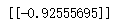
b,alphas = smoP(dataMat,labelMat, 0.6, 0.001, 40)

print(b)

print(alphas[alphas>0])

下面列出的一个小函数可
以用于实现上述任务：

def calcWs(alphas,dataArr,classLabels):

    X = mat(dataArr); labelMat = mat(classLabels).transpose()

    m,n = shape(X)

    w = zeros((n,1))

    for i in range(m):

        w += multiply(alphas[i]*labelMat[i],X[i,:].T)

    return w

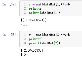
w = calcWs(alphas,dataMat,labelMat)

print(w)

r = mat(dataMat[0])*w+b

print(r)

print(labelMat[0])

利用核函数将数据映射到高维空间

数据点处于一个圆中，人类的大脑能够意识到这一点。然而，对于分类器而言，
它只能识别分类器的结果是大于0还是小于0。如果只在1和^轴构成的坐标系中插人直线进行分类
的话，我们并不会得到理想的结果。我们或许可以对圆中的数据进行某种形式的转换，从而得到
某些新的变量来表示数据。在这种表示情况下，我们就更容易得到大于0或者小于0的测试结果。
在这个例子中，我们将数据从一个特征空间转换到另一个特征空间。在新空间下，我们可以很容
易利用巳有的工具对数据进行处理。数学家们喜欢将这个过程称之为从一个特征空间到另一个特
择空间的映射。在通常情况下，这种映射会将低维特征空间映射到高维空间。

这种从某个特征空间到另一个特征空间的映射是通过核函数来实现的。

核函数并不仅仅应用于支持向量机，很多其他的机器学习算法也都用到核函数。

径向基核函数

上述高斯核函数将数据从其特征空间映射到更高维的空间，具体来说这里是映射到一个无穷
维的空间。

高斯核函数只是一个常用的核函数，使用
者并不需要确切地理解数据到底是如何表现的，而且使用高斯核函数还会得到一个理想的结果。

def kernelTrans(X, A, kTup): #calc the kernel or transform data to a higher dimensional space

    m,n = shape(X)

    K = mat(zeros((m,1)))

    if kTup[0]=='lin':

        K = X * A.T   #linear kernel

    elif kTup[0]=='rbf':

        for j in range(m):

            deltaRow = X[j,:] - A

            K[j] = deltaRow*deltaRow.T

        K = exp(K/(-1*kTup[1]**2)) #divide in NumPy is element-wise not matrix like Matlab

    else: raise NameError('Houston We Have a Problem -- That Kernel is not recognized')

    return K

在测试中使用核函数

利用核函数进行分类的径向基测试函数

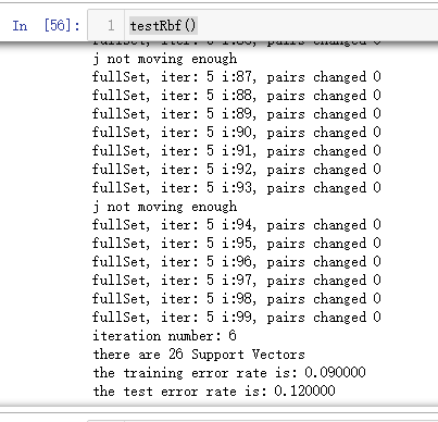
def testRbf(k1=1.3):

    dataArr,labelArr = loadDataSet('F:\\machinelearninginaction\\Ch06\\testSetRBF.txt')

    b,alphas = smoP(dataArr, labelArr, 200, 0.0001, 10000, ('rbf', k1)) #C=200 important

    datMat=mat(dataArr); labelMat = mat(labelArr).transpose()

    svInd=nonzero(alphas.A>0)[0]

    sVs=datMat[svInd] #get matrix of only support vectors

    labelSV = labelMat[svInd];

    print("there are %d Support Vectors" % shape(sVs)[0])

    m,n = shape(datMat)

    errorCount = 0

    for i in range(m):

        kernelEval = kernelTrans(sVs,datMat[i,:],('rbf', k1))

        predict=kernelEval.T * multiply(labelSV,alphas[svInd]) + b

        if sign(predict)!=sign(labelArr[i]):

            errorCount += 1

    print("the training error rate is: %f" % (float(errorCount)/m))

    dataArr,labelArr = loadDataSet('F:\\machinelearninginaction\\Ch06\\testSetRBF2.txt')

    errorCount = 0

    datMat=mat(dataArr)

    labelMat = mat(labelArr).transpose()

    m,n = shape(datMat)

    for i in range(m):

        kernelEval = kernelTrans(sVs,datMat[i,:],('rbf', k1))

        predict=kernelEval.T * multiply(labelSV,alphas[svInd]) + b

        if sign(predict)!=sign(labelArr[i]):

            errorCount += 1

    print("the test error rate is: %f" % (float(errorCount)/m))

巴特西

吴裕雄--天生自然python机器学习：支持向量机SVM

最新文章

热门文章