pytorch学习笔记四之训练分类器
训练分类器
1. 数据
处理图像,文本,音频或视频数据时,可以使用将数据加载到 NumPy 数组中的标准 Python 包。 然后,将该数组转换为torch.*Tensor
- 对于图像,Pillow,OpenCV 等包很有用
- 对于音频,请使用 SciPy 和 librosa 等包
- 对于文本,基于 Python 或 Cython 的原始加载,或者 NLTK 和 SpaCy 很有用
专门针对视觉,一个名为torchvision的包,其中包含用于常见数据集(例如 Imagenet,CIFAR10,MNIST 等)的数据加载器,以及用于图像(即torchvision.datasets和torch.utils.data.DataLoader)的数据转换器
我们将使用 CIFAR10 数据集。 它具有以下类别:“飞机”,“汽车”,“鸟”,“猫”,“鹿”,“狗”,“青蛙”,“马”,“船”,“卡车”。 CIFAR-10 中的图像尺寸为3x32x32,即尺寸为32x32像素的 3 通道彩色图像
数据集来源:CIFAR-10 and CIFAR-100 datasets
| airplane |  |
 |
 |
 |
 |
 |
 |
 |
 |
 |
| automobile |  |
 |
 |
 |
 |
 |
 |
 |
 |
 |
| bird |  |
 |
 |
 |
 |
 |
 |
 |
 |
 |
| cat |  |
 |
 |
 |
 |
 |
 |
 |
 |
 |
| deer |  |
 |
 |
 |
 |
 |
 |
 |
 |
 |
| dog |  |
 |
 |
 |
 |
 |
 |
 |
 |
 |
| frog |  |
 |
 |
 |
 |
 |
 |
 |
 |
 |
| horse |  |
 |
 |
 |
 |
 |
 |
 |
 |
 |
| ship |  |
 |
 |
 |
 |
 |
 |
 |
 |
 |
| truck |  |
 |
 |
 |
 |
 |
 |
 |
 |
 |
由于图片地址在国外,以上图片的加载可能不如人意,大致就是这个图像: 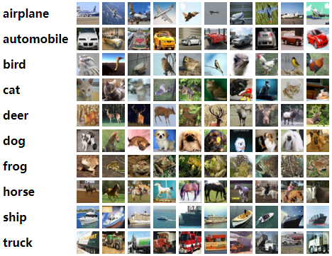
2. 训练一个分类器
我们将会按顺序做以下步骤:
- 用torchvision 加载和标准化CIFAR10训练和测试数据
- 定义一个神经网络
- 定义一个损失函数
- 使用训练数据训练网络
- 使用测试数据测试网络
2.1. 加载数据并标准化
使用torchvision加载CIFAR10数据十分简单:
import torch

import torchvision

import torchvision.transforms as transforms
输出的torchvision数据集是PILImage图像,其范围是[0,1]。我们将它转化为Tensor的标准范围[-1,1]
transform = transforms.Compose(

    [transforms.ToTensor(),

     transforms.Normalize((0.5, 0.5, 0.5), (0.5, 0.5, 0.5))])

batch_size = 4

trainset = torchvision.datasets.CIFAR10(root='./data', train=True,

                                        download=True, transform=transform)

trainloader = torch.utils.data.DataLoader(trainset, batch_size=batch_size,

                                          shuffle=True, num_workers=0)

testset = torchvision.datasets.CIFAR10(root='./data', train=False,

                                       download=True, transform=transform)

testloader = torch.utils.data.DataLoader(testset, batch_size=batch_size,

                                         shuffle=False, num_workers=0)

classes = ('plane', 'car', 'bird', 'cat',

           'deer', 'dog', 'frog', 'horse', 'ship', 'truck')
Files already downloaded and verified

Files already downloaded and verified
- 注意:如果在Windows上运行并且得到BrankPipeError,请尝试将Torch.utils.Data.Dataloader()的Num_Worker设置为0。官网示例是Num_Worker设置为2
让我们显示一下训练的图片:
import matplotlib.pyplot as plt

import numpy as np

# functions to show an image

def imshow(img):

    img = img / 2 + 0.5     # unnormalize

    npimg = img.numpy()

    plt.imshow(np.transpose(npimg, (1, 2, 0)))

    plt.show()

# get some random training images

dataiter = iter(trainloader)

images, labels = dataiter.next()

# show images

imshow(torchvision.utils.make_grid(images))

# print labels

print(' '.join(f'{classes[labels[j]]:5s}' for j in range(batch_size)))
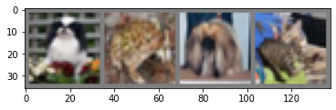
dog frog dog cat
2.2.定义一个卷积神经网络
import torch.nn as nn

import torch.nn.functional as F

class Net(nn.Module):

    def __init__(self):

        super().__init__()

        self.conv1 = nn.Conv2d(3, 6, 5)

        self.pool = nn.MaxPool2d(2, 2)

        self.conv2 = nn.Conv2d(6, 16, 5)

        self.fc1 = nn.Linear(16 * 5 * 5, 120)

        self.fc2 = nn.Linear(120, 84)

        self.fc3 = nn.Linear(84, 10)

    def forward(self, x):

        x = self.pool(F.relu(self.conv1(x)))

        x = self.pool(F.relu(self.conv2(x)))

        x = torch.flatten(x, 1) # flatten all dimensions except batch

        x = F.relu(self.fc1(x))

        x = F.relu(self.fc2(x))

        x = self.fc3(x)

        return x

net = Net()
2.3.定义一个损失函数和优化器
让我们使用分类交叉熵损失和带有动量的 SGD
import torch.optim as optim

criterion = nn.CrossEntropyLoss()

optimizer = optim.SGD(net.parameters(), lr=0.001, momentum=0.9)
2.4.训练网络
有趣的事情开始了,我们只需要循环我们的迭代器,并反馈到网络进行优化
for epoch in range(2):  # loop over the dataset multiple times

    running_loss = 0.0

    for i, data in enumerate(trainloader, 0):

        # get the inputs; data is a list of [inputs, labels]

        inputs, labels = data

        # zero the parameter gradients

        optimizer.zero_grad()

        # forward + backward + optimize

        outputs = net(inputs)

        loss = criterion(outputs, labels)

        loss.backward()

        optimizer.step()

        # print statistics

        running_loss += loss.item()

        if i % 2000 == 1999:    # print every 2000 mini-batches

            print(f'[{epoch + 1}, {i + 1:5d}] loss: {running_loss / 2000:.3f}')

            running_loss = 0.0

print('Finished Training')
[1,  2000] loss: 2.193

[1,  4000] loss: 1.847

[1,  6000] loss: 1.661

[1,  8000] loss: 1.569

[1, 10000] loss: 1.488

[1, 12000] loss: 1.445

[2,  2000] loss: 1.405

[2,  4000] loss: 1.355

[2,  6000] loss: 1.329

[2,  8000] loss: 1.320

[2, 10000] loss: 1.277

[2, 12000] loss: 1.250

Finished Training
快速保存训练模型:
PATH = './cifar_net.pth'

torch.save(net.state_dict(), PATH)
2.5.使用测试集测试网络
显示测试集中的图像:
dataiter = iter(testloader)

images, labels = dataiter.next()

# print images

imshow(torchvision.utils.make_grid(images))

print('GroundTruth: ', ' '.join(f'{classes[labels[j]]:5s}' for j in range(4)))
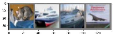
GroundTruth: cat ship ship plane
加载保存的模型:
net = Net()

net.load_state_dict(torch.load(PATH))
<All keys matched successfully>使用神经网络进行预测:
outputs = net(images)
outputs
tensor([[-0.4519, -2.6896,  1.1111,  2.4411, -1.2739,  0.9407,  1.2027, -0.9218,

         -0.3061, -1.4944],

        [ 4.0095,  5.7177, -1.3274, -3.2596, -4.4239, -6.4377, -5.2835, -5.2639,

          8.8550,  3.4490],

        [ 2.2643,  1.9055,  0.2977, -1.2159, -1.5517, -2.6117, -2.5904, -2.0696,

          3.1488,  0.7971],

        [ 3.6302,  0.2553,  0.3926, -1.3850,  0.2644, -2.8077, -2.8192, -1.0332,

          1.9776,  0.4094]], grad_fn=<AddmmBackward0>)
输出是 10 类的能量。 一个类别的能量越高,网络就认为该图像属于特定类别。 因此,让我们获取最高能量的指数:
_, predicted = torch.max(outputs, 1)

print('Predicted: ', ' '.join(f'{classes[predicted[j]]:5s}'

                              for j in range(4)))
Predicted: cat ship ship plane
此次结果看起来不错
我们看看这个网络在整个数据集的表现:
correct = 0

total = 0

# since we're not training, we don't need to calculate the gradients for our outputs

with torch.no_grad():

    for data in testloader:

        images, labels = data

        # calculate outputs by running images through the network

        outputs = net(images)

        # the class with the highest energy is what we choose as prediction

        _, predicted = torch.max(outputs.data, 1)

        total += labels.size(0)

        correct += (predicted == labels).sum().item()

print(f'Accuracy of the network on the 10000 test images: {100 * correct // total} %')
Accuracy of the network on the 10000 test images: 56 %
这看起来是比偶然更好(偶然的准确率是10%,即从10个类别中选择一个),看起来这个网络学到了一些东西
看看这个这个分类器在哪些类别分类好,哪些类别分类差:
# prepare to count predictions for each class

correct_pred = {classname: 0 for classname in classes}

total_pred = {classname: 0 for classname in classes}

# again no gradients needed

with torch.no_grad():

    for data in testloader:

        images, labels = data

        outputs = net(images)

        _, predictions = torch.max(outputs, 1)

        # collect the correct predictions for each class

        for label, prediction in zip(labels, predictions):

            if label == prediction:

                correct_pred[classes[label]] += 1

            total_pred[classes[label]] += 1

# print accuracy for each class

for classname, correct_count in correct_pred.items():

    accuracy = 100 * float(correct_count) / total_pred[classname]

    print(f'Accuracy for class: {classname:5s} is {accuracy:.1f} %')
Accuracy for class: plane is 65.5 %

Accuracy for class: car   is 67.1 %

Accuracy for class: bird  is 30.4 %

Accuracy for class: cat   is 53.5 %

Accuracy for class: deer  is 44.2 %

Accuracy for class: dog   is 35.9 %

Accuracy for class: frog  is 68.2 %

Accuracy for class: horse is 70.3 %

Accuracy for class: ship  is 68.9 %

Accuracy for class: truck is 60.4 %
2.6.在GPU上训练
如果可以使用 CUDA,首先将我们的设备定义为第一个可见的 cuda 设备:
device = torch.device('cuda:0' if torch.cuda.is_available() else 'cpu')

# Assuming that we are on a CUDA machine, this should print a CUDA device:

print(device)
cuda:0
然后,这些方法将递归遍历所有模块,并将其参数和缓冲区转换为 CUDA 张量:
net.to(device)
Net(

  (conv1): Conv2d(3, 6, kernel_size=(5, 5), stride=(1, 1))

  (pool): MaxPool2d(kernel_size=2, stride=2, padding=0, dilation=1, ceil_mode=False)

  (conv2): Conv2d(6, 16, kernel_size=(5, 5), stride=(1, 1))

  (fc1): Linear(in_features=400, out_features=120, bias=True)

  (fc2): Linear(in_features=120, out_features=84, bias=True)

  (fc3): Linear(in_features=84, out_features=10, bias=True)

)
还必须将每一步的输入和目标也发送到 GPU:
inputs, labels = data[0].to(device), data[1].to(device)
3.参考资料
[2]训练分类器
最新文章
- the operation was attempted on an empty geometry Arcgis Project异常
- 基于C/S架构的3D对战网络游戏C++框架 _02系统设计(总体设计、概要设计)
- go2shell的安装与修改默认terminal方法
- Windows下查看端口占用
- 十二、BOOL冒泡
- Oracle 关于定义约束 / 修改表结构 /修改约束
- 关于百度地图API的地图坐标转换问题
- login-登录
- (转)[老老实实学WCF] 第一篇 Hello WCF
- PHP不显示报错了怎么办~
- JS计算字符串长度(中文算2个)
- 201521123093 JAVA程序设计
- poi导入Excel,数字科学记数法转换
- Hadoop记录- Yarn scheduler队列采集
- requestium
- 前端lvs访问多台nginx代理服务时出现404错误的处理
- QPS、PV 、RT(响应时间)之间的关系
- 在mk/rte.app.mk 256行加echo $(O_TO_EXE_DO)查看GCC参数
- oracle数据库之操作总结
- jQuery瀑布流无限拖三大利器:masonry+imagesloaded+infinitescroll