# ----------------------------------------------------#

# R in Action (2nd ed): Chapter 3                     #

# Getting started with graphs                         #

# requires that the Hmisc and RColorBrewer  packages  #

# have been installed                                 #

# install.packages(c("Hmisc", "RColorBrewer"))        #

#-----------------------------------------------------#

par(ask=TRUE)

opar <- par(no.readonly=TRUE) # make a copy of current settings

attach(mtcars) # be sure to execute this line

plot(wt, mpg)

abline(lm(mpg~wt))

title("Regression of MPG on Weight")

# Input data for drug example

dose  <- c(20, 30, 40, 45, 60)

drugA <- c(16, 20, 27, 40, 60)

drugB <- c(15, 18, 25, 31, 40)

plot(dose, drugA, type="b")

opar <- par(no.readonly=TRUE) # make a copy of current settings

par(lty=2, pch=17)            # change line type and symbol

plot(dose, drugA, type="b")   # generate a plot

par(opar)                     # restore the original settings 

plot(dose, drugA, type="b", lty=3, lwd=3, pch=15, cex=2)

# choosing colors

library(RColorBrewer)

n <- 7

mycolors <- brewer.pal(n, "Set1")

barplot(rep(1,n), col=mycolors)

n <- 10

mycolors <- rainbow(n)

pie(rep(1, n), labels=mycolors, col=mycolors)

mygrays <- gray(0:n/n)

pie(rep(1, n), labels=mygrays, col=mygrays)

# Listing 3.1 - Using graphical parameters to control graph appearance

dose <- c(20, 30, 40, 45, 60)

drugA <- c(16, 20, 27, 40, 60)

drugB <- c(15, 18, 25, 31, 40)

opar <- par(no.readonly=TRUE)

par(pin=c(2, 3))

par(lwd=2, cex=1.5)

par(cex.axis=.75, font.axis=3)

plot(dose, drugA, type="b", pch=19, lty=2, col="red")

plot(dose, drugB, type="b", pch=23, lty=6, col="blue", bg="green")

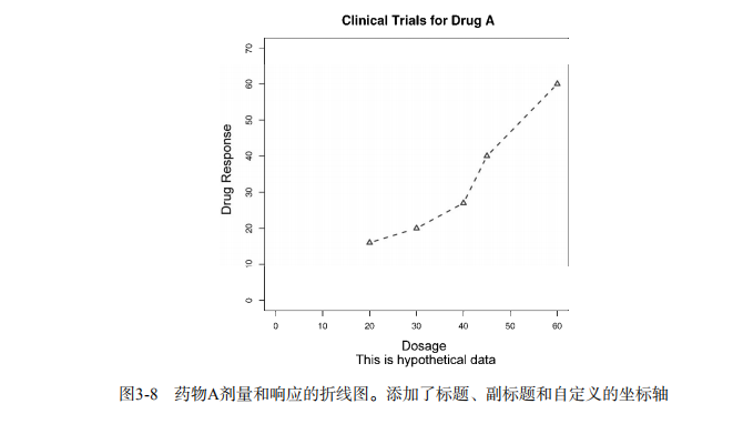
par(opar)                

# Adding text, lines, and symbols

plot(dose, drugA, type="b",

     col="red", lty=2, pch=2, lwd=2,

     main="Clinical Trials for Drug A",

     sub="This is hypothetical data",

     xlab="Dosage", ylab="Drug Response",

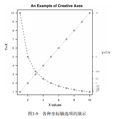
     xlim=c(0, 60), ylim=c(0, 70))

# Listing 3.2 - An Example of Custom Axes

x <- c(1:10)

y <- x

z <- 10/x

opar <- par(no.readonly=TRUE)

par(mar=c(5, 4, 4, 8) + 0.1)

plot(x, y, type="b",

     pch=21, col="red",

     yaxt="n", lty=3, ann=FALSE)

lines(x, z, type="b", pch=22, col="blue", lty=2)

axis(2, at=x, labels=x, col.axis="red", las=2)

axis(4, at=z, labels=round(z, digits=2),

     col.axis="blue", las=2, cex.axis=0.7, tck=-.01)

mtext("y=1/x", side=4, line=3, cex.lab=1, las=2, col="blue")

title("An Example of Creative Axes",

      xlab="X values",

      ylab="Y=X")

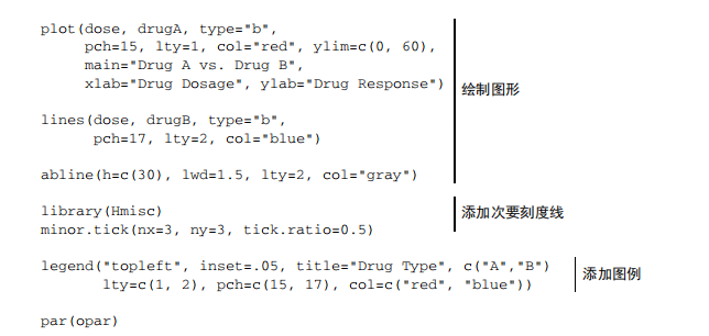
par(opar)

# Listing 3.3 - Comparing Drug A and Drug B response by dose

dose <- c(20, 30, 40, 45, 60)

drugA <- c(16, 20, 27, 40, 60)

drugB <- c(15, 18, 25, 31, 40)

opar <- par(no.readonly=TRUE)

par(lwd=2, cex=1.5, font.lab=2)

plot(dose, drugA, type="b",

     pch=15, lty=1, col="red", ylim=c(0, 60),

     main="Drug A vs. Drug B",

     xlab="Drug Dosage", ylab="Drug Response")

lines(dose, drugB, type="b",

      pch=17, lty=2, col="blue")

abline(h=c(30), lwd=1.5, lty=2, col="gray")

library(Hmisc)

minor.tick(nx=3, ny=3, tick.ratio=0.5)

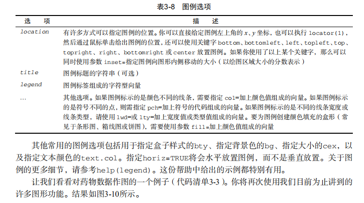
legend("topleft", inset=.05, title="Drug Type", c("A","B"),

       lty=c(1, 2), pch=c(15, 17), col=c("red", "blue"))

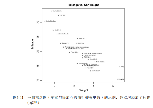
par(opar)

# Example of labeling points

attach(mtcars)

plot(wt, mpg,

     main="Mileage vs. Car Weight",

     xlab="Weight", ylab="Mileage",

     pch=18, col="blue")

text(wt, mpg,

     row.names(mtcars),

     cex=0.6, pos=4, col="red")

detach(mtcars)

# View font families

opar <- par(no.readonly=TRUE)

par(cex=1.5)

plot(1:7,1:7,type="n")

text(3,3,"Example of default text")

text(4,4,family="mono","Example of mono-spaced text")

text(5,5,family="serif","Example of serif text")

par(opar)

# Combining graphs

attach(mtcars)

opar <- par(no.readonly=TRUE)

par(mfrow=c(2,2))

plot(wt,mpg, main="Scatterplot of wt vs. mpg")

plot(wt,disp, main="Scatterplot of wt vs. disp")

hist(wt, main="Histogram of wt")

boxplot(wt, main="Boxplot of wt")

par(opar)

detach(mtcars)

attach(mtcars)

opar <- par(no.readonly=TRUE)

par(mfrow=c(3,1))

hist(wt)

hist(mpg)

hist(disp)

par(opar)

detach(mtcars)

attach(mtcars)

layout(matrix(c(1,1,2,3), 2, 2, byrow = TRUE))

hist(wt)

hist(mpg)

hist(disp)

detach(mtcars)

attach(mtcars)

layout(matrix(c(1, 1, 2, 3), 2, 2, byrow = TRUE),

       widths=c(3, 1), heights=c(1, 2))

hist(wt)

hist(mpg)

hist(disp)

detach(mtcars)

# Listing 3.4 - Fine placement of figures in a graph

opar <- par(no.readonly=TRUE)

par(fig=c(0, 0.8, 0, 0.8))

plot(mtcars$mpg, mtcars$wt,

     xlab="Miles Per Gallon",

     ylab="Car Weight")

par(fig=c(0, 0.8, 0.55, 1), new=TRUE)

boxplot(mtcars$mpg, horizontal=TRUE, axes=FALSE)

par(fig=c(0.65, 1, 0, 0.8), new=TRUE)

boxplot(mtcars$wt, axes=FALSE)

mtext("Enhanced Scatterplot", side=3, outer=TRUE, line=-3)

par(opar)