前言

最近在youtube 上学习CS231n的课程，并尝试完成Assgnments,收获很多，这里记录下过程和结果以及过程中遇到的问题，我并不是只是完成需要补充的代码段，对于自己不熟悉的没用过的库函数查了官方文档，并做了注释，每个Assignments 完成后，我会将代码会放到我的GitHub。Assignments 1 is here

在本地完成，需要从这里下载数据，将cifar-10-batches-py文件夹解压到cs231n/datasets 下

Q1-1 k-Nearest Neighbor (kNN) exercise

1.import Lib

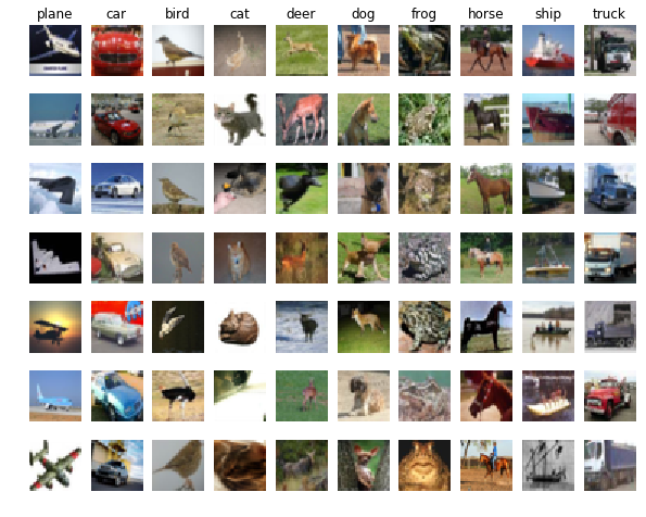
2.load data and print data info and show some data

这里有一个enumerate() 函数 ## 用于将一个可遍历的数据对象(如列表、元组或字符串)组合为一个索引序列，同时列出数据和数据下标。我以前用过unique()函数来返回value and index,对这个函数忘记了

3.process data :Reshape the image data into rows

4. realize the KNN and use KNN method to classify

create KNN classifier object

remember that we do not need to anthing for the KNN,,the Classifier simply remembers the data and does no further processing

We would now like to classify the test data with the kNN classifier. Recall that we can break down this process into two steps:

First we must compute the distances between all test examples and all train examples.
Given these distances, for each test example we find the k nearest examples and have them vote for the label

here we will use three methods to compute the distance between X_train data and X_test data

method 1. compute_distance_two_loop

Compute the distance between each test point in X and each training point in self.X_train using a nested loop over both the training data and the test data.

def compute_distances_two_loops(self, X):

    """

    Compute the distance between each test point in X and each training point

    in self.X_train using a nested loop over both the training data and the

    test data.

    Inputs:

    - X: A numpy array of shape (num_test, D) containing test data.

    Returns:

    - dists: A numpy array of shape (num_test, num_train) where dists[i, j]

      is the Euclidean distance between the ith test point and the jth training

      point.

    """

    num_test = X.shape[0]

    num_train = self.X_train.shape[0]

    dists = np.zeros((num_test, num_train))

    for i in xrange(num_test):

      for j in xrange(num_train):

        #####################################################################

        # TODO:                                                             #

        # Compute the l2 distance between the ith test point and the jth    #

        # training point, and store the result in dists[i, j]. You should   #

        # not use a loop over dimension.                                    #

        #####################################################################

        #pass

        dists[i,j] = np.sqrt(np.sum(np.square(self.X_train[j,:]-X[i,:])))

        #####################################################################

        #                       END OF YOUR CODE                            #

        #####################################################################

    return dists

we can visualize the distance matrix: each row is a single test example and its distances to training examples

then we compete the predict_label

def predict_labels(self, dists, k=1):

    """

    Given a matrix of distances between test points and training points,

    predict a label for each test point.

    Inputs:

    - dists: A numpy array of shape (num_test, num_train) where dists[i, j]

      gives the distance betwen the ith test point and the jth training point.

    Returns:

    - y: A numpy array of shape (num_test,) containing predicted labels for the

      test data, where y[i] is the predicted label for the test point X[i].

    """

    num_test = dists.shape[0]

    y_pred = np.zeros(num_test)

    for i in xrange(num_test):

      # A list of length k storing the labels of the k nearest neighbors to

      # the ith test point.

      closest_y = []

      #########################################################################

      # TODO:                                                                 #

      # Use the distance matrix to find the k nearest neighbors of the ith    #

      # testing point, and use self.y_train to find the labels of these       #

      # neighbors. Store these labels in closest_y.                           #

      # Hint: Look up the function numpy.argsort.                             #

      #########################################################################

      #pass

      closest_y = self.y_train[np.argsort(dists[i][:k])]

      #########################################################################

      # TODO:                                                                 #

      # Now that you have found the labels of the k nearest neighbors, you    #

      # need to find the most common label in the list closest_y of labels.   #

      # Store this label in y_pred[i]. Break ties by choosing the smaller     #

      # label.                                                                #

      #########################################################################

      #pass

      y_pred[i] = np.argmax(np.bincount(closest_y))

      #########################################################################

      #                           END OF YOUR CODE                            #

      #########################################################################

    return y_pred

here given a hint: use the numpy.argsort(),I search the document :numpy.argsort(a, axis=-1, kind='quicksort', order=None)[source] Returns the indices that would sort an array.

our first trest setting K =1 and its accuracy is Got 54 / 500 correct => accuracy: 0.108000 ,I do not know why is much lower than the offical answer, I am sure the method is right

the set K =5,it is a little higher than K=1, Got 56 / 500 correct => accuracy: 0.112000

method 2.compute_distances_one_loop

 def compute_distances_one_loop(self, X):

     """

     Compute the distance between each test point in X and each training point

     in self.X_train using a single loop over the test data.

     Input / Output: Same as compute_distances_two_loops

     """

     num_test = X.shape[0]

     num_train = self.X_train.shape[0]

     dists = np.zeros((num_test, num_train))

     for i in xrange(num_test):

       #######################################################################

       # TODO:                                                               #

       # Compute the l2 distance between the ith test point and all training #

       # points, and store the result in dists[i, :].                        #

       #######################################################################

       #pass

       dists[i,:] = np.sqrt(np.sum(np.square(self.X_train-X[i,:]),axis =1))

       #######################################################################

       #                         END OF YOUR CODE                            #

       #######################################################################

     return dists

# To ensure that our vectorized implementation is correct, we make sure that it agrees with the naive implementation. There are many ways to decide whether two matrices are similar; one of the simplest is the Frobenius norm ( if forget the F-norm,reference the Matrix Analisis)

the result is :same Difference was: 0.000000 Good! The distance matrices are the same

method 3 compute_distances_no_loops (implement the fully vectorized version inside compute_distances_no_loops)

here give a hint : Try to formulate the l2 distance using matrix multiplication and two broadcast sums.

give the code first

 def compute_distances_no_loops(self, X):

     """

     Compute the distance between each test point in X and each training point

     in self.X_train using no explicit loops.

     Input / Output: Same as compute_distances_two_loops

     """

     num_test = X.shape[0]

     num_train = self.X_train.shape[0]

     dists = np.zeros((num_test, num_train))

     #########################################################################

     # TODO:                                                                 #

     # Compute the l2 distance between all test points and all training      #

     # points without using any explicit loops, and store the result in      #

     # dists.                                                                #

     #                                                                       #

     # You should implement this function using only basic array operations; #

     # in particular you should not use functions from scipy.                #

     #                                                                       #

     # HINT: Try to formulate the l2 distance using matrix multiplication    #

     #       and two broadcast sums.                                         #

     #########################################################################

     #pass

     dists = np.multiply(np.dot(X,self.X_train.T),-2)

     sq1 = np.sum(np.square(X),axis=1,keepdims = True)

     sq2 = np.sum(np.square(self.X_train),axis =1)

     dists = np.add(dists,sq1)

     dists = np.add(dists,sq2)

     dists = np.sqrt(dists)

     #########################################################################

     #                         END OF YOUR CODE                              #

     #########################################################################

     return dists

I will explain this method following

we know tha train data and tha test data has the same type ,they just have different number samples,

Assume that our train data is and test data is ,the square of distances of the them is matrix

we can compute the ,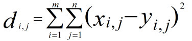，we can not use loop ,so we could not use this formular directly,the hint tell us we can use the matrix multilpy,when to use the multiply function ,multiply will come out when Complete square formula expansion ,so 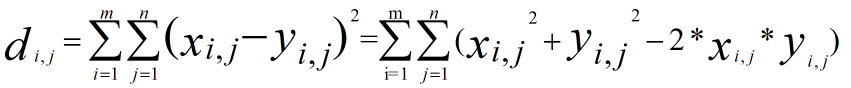,the lthird item can use the multiply,the top second should use the sum(square()),I give the examples for the computing process .

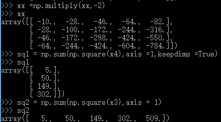
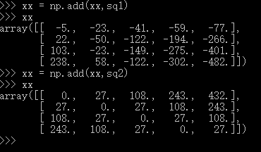
suggestion:if you do not understand some process ,you can use list some examples and run it in the python interactive environment

Q1-2 Multiclass Support Vector Machine exercise

similar to Q1-1

1.first:,load the data,

prtint the data shape,

 Training data shape:  (50000, 32, 32, 3)

 Training labels shape:  (50000,)

 Test data shape:  (10000, 32, 32, 3)

 Test labels shape:  (10000,)

show some samples

2.split the data to train data ,validation data and test data

 Train data shape:  (49000, 32, 32, 3)

 Train labels shape:  (49000,)

 Validation data shape:  (1000, 32, 32, 3)

 Validation labels shape:  (1000,)

 Test data shape:  (1000, 32, 32, 3)

 Test labels shape:  (1000,)

 Training data shape:  (49000, 3072)

 Validation data shape:  (1000, 3072)

 Test data shape:  (1000, 3072)

 dev data shape:  (500, 3072)

3.data processing,

reshape the data to 2D,
minus the mean of the images

4.SVM Classifier

Loss Function

gradient with calsulus and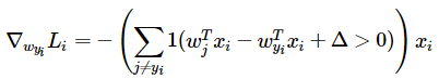

the function svm_loss_naive(W, X, y, reg) in linear_svm.py realize the functions above use loop,the code as follows:

 def svm_loss_naive(W, X, y, reg):

   """

   Structured SVM loss function, naive implementation (with loops).

   Inputs have dimension D, there are C classes, and we operate on minibatches

   of N examples.

   Inputs:

   - W: A numpy array of shape (D, C) containing weights.

   - X: A numpy array of shape (N, D) containing a minibatch of data.

   - y: A numpy array of shape (N,) containing training labels; y[i] = c means

     that X[i] has label c, where 0 <= c < C.

   - reg: (float) regularization strength

   Returns a tuple of:

   - loss as single float

   - gradient with respect to weights W; an array of same shape as W

   """

   dW = np.zeros(W.shape) # initialize the gradient as zero

   # compute the loss and the gradient

   num_classes = W.shape[1]

   num_train = X.shape[0]

   loss = 0.0

   for i in xrange(num_train):

     scores = X[i].dot(W)

     correct_class_score = scores[y[i]]

     for j in xrange(num_classes):

       if j == y[i]:

         continue

       margin = scores[j] - correct_class_score + 1 # note delta = 1

       if margin > 0:

         loss += margin

         dW[:,y[i]] +=-X[i,:].T

         dW[:,j]+=X[i,:].T

   # Right now the loss is a sum over all training examples, but we want it

   # to be an average instead so we divide by num_train.

   loss /= num_train

   dW  /=num_train

   # Add regularization to the loss.

   loss += reg * np.sum(W * W)

   dW +=reg*W

then call the function above int the note book and print the loss ,the loss : loss: 9.028430 ,

5.check the gradient

To check that you have correctly implemented the gradient correctly, you can numerically estimate the gradient of the loss function and compare the numeric estimate to the gradient that you computed.

output:

in order to distinguish between adding the reg and no regulartion ,I print a line to note

 numerical: 4.390430 analytic: 4.432183, relative error: 4.732604e-03

 numerical: 0.744468 analytic: 0.744468, relative error: 1.921408e-10

 numerical: -30.520313 analytic: -30.520313, relative error: 1.419558e-13

 numerical: -2.132037 analytic: -2.132037, relative error: 7.127561e-11

 numerical: -18.507272 analytic: -18.507272, relative error: 4.874040e-12

 numerical: 8.862828 analytic: 8.862828, relative error: 1.344790e-11

 numerical: -0.170896 analytic: -0.170896, relative error: 7.526124e-10

 numerical: -9.717059 analytic: -9.717059, relative error: 2.095593e-11

 numerical: -5.810426 analytic: -5.810426, relative error: 4.130797e-11

 numerical: 8.401579 analytic: 8.401579, relative error: 1.702498e-11

 add the regulartion

 numerical: -2.239516 analytic: -2.258984, relative error: 4.327772e-03

 numerical: 10.431021 analytic: 10.432692, relative error: 8.009829e-05

 numerical: -6.335932 analytic: -6.342876, relative error: 5.476725e-04

 numerical: 8.736775 analytic: 8.751631, relative error: 8.494921e-04

 numerical: 9.121414 analytic: 9.123640, relative error: 1.220078e-04

 numerical: -0.485200 analytic: -0.485900, relative error: 7.204892e-04

 numerical: -1.188862 analytic: -1.187261, relative error: 6.737057e-04

 numerical: -4.172487 analytic: -4.169791, relative error: 3.230742e-04

 numerical: -17.164400 analytic: -17.156470, relative error: 2.310661e-04

 numerical: 19.665208 analytic: 19.666977, relative error: 4.498910e-05

Inline Question 1:

It is possible that once in a while a dimension in the gradcheck will not match exactly. What could such a discrepancy be caused by? Is it a reason for concern? What is a simple example in one dimension where a gradient check could fail? Hint: the SVM loss function is not strictly speaking differentiable

Answer: from the output,we can see that,except the first line,the relative error is much larger than the others in the kind of not adding the regulartion,All of the others are close to each other.

So, the reason that the big difference of the first one beacuse ,Numerical solution is an approximation solution,when it is nondifferentia at some points of the Loss function,the two solutions will be different.

6.implement the function svm_loss_vectorized

finish the function svm_loss_vectorized(W,Y,y,reg) in the linear_svm.py

the code as follows:

 def svm_loss_vectorized(W, X, y, reg):

   """

   Structured SVM loss function, vectorized implementation.

   Inputs and outputs are the same as svm_loss_naive.

   """

   loss = 0.0

   dW = np.zeros(W.shape) # initialize the gradient as zero

   #############################################################################

   # TODO:                                                                     #

   # Implement a vectorized version of the structured SVM loss, storing the    #

   # result in loss.                                                           #

   #############################################################################

   #pass

   scores = X.dot(W)

   num_classes = W.shape[1]

   num_train = X.shape[0]

   scores_correct = scores[np.arange(num_train),y]

   scores_correct = np.reshape(scores_correct,(num_train,-1))

   margins = scores - scores_correct+1

   margins = np.maximum(0,margins)

   margins[np.arange(num_train),y]=0

   loss += np.sum(margins)/num_train

   loss +=0.5*reg*np.sum(W*W)

   #############################################################################

   #                             END OF YOUR CODE                              #

   #############################################################################

   #############################################################################

   # TODO:                                                                     #

   # Implement a vectorized version of the gradient for the structured SVM     #

   # loss, storing the result in dW.                                           #

   #                                                                           #

   # Hint: Instead of computing the gradient from scratch, it may be easier    #

   # to reuse some of the intermediate values that you used to compute the     #

   # loss.                                                                     #

   #############################################################################

   #pass

   margins[margins >0] =1

   row_sum = np.sum(margins,axis =1)

   margins[np.arange(num_train),y] = -row_sum

   dW +=np.dot(X.T,margins)/num_train +reg*W

   #############################################################################

   #                             END OF YOUR CODE                              #

   #############################################################################

   return loss, dW

这里记录一下，在完成这个函数的时候遇到的问题，我们使用X 与W的点乘得到了所有的scores，但是，我需要将每一个class对应的score选择出来，而我们不能使用循环，即不能使用下标运算，此时，我们可以看一下score，这是一个矩阵，每一列对应一个类别，

虽然，不是对称矩阵，但已然可以认为对角线的元素对应每个example的正确class的score,那就需要两个分别表示行和列的index的一维数组，我们知道在numpy中是可以这样使用的，就以上面这个scores的矩阵，scores[0,0],[1,1]....[num_train-1,y],那就可以以这两个构造index，当然，我上边这个不合理，我一共有5个样本，三个类别，那我的y也必须是(5,),这样用scores选则的时候会出现边界错误，再更正一下，上面的是合理的，6个类别，当然，5个样本，6个类别，实际情况是不是很合理，但是对于理解问题，没有影响，我最初据的例子是三个类别，会出现 IndexError: index 3 is out of bounds for axis 1 with size 3 ，当然，这个很容易找到错误原因，所以，我立刻修改了W的维数参数，数据当然不合理，主要还是因为目前我练习的项目还少，向量化不会很直觉的就写出来，就在交互式环境中看看自己的想法是不是对，拿这个例子来说，我分别造出X 和W 来可视化我的理解，

大致过程如下：

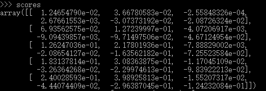
构造X， X_tr = np.arange(240).reshape((5,4,4,3)) ，这里我就给出X_tr 的详细结果了，一共240个数，已经很容易理解了，然后转成二维的 X_tr =np.hstack([X_tr,np.ones((X_tr.shape[0],1))]) ，

然后，加一个bias,

这里，我只显示了前2行，现在造W , W = np.random.randn(X_tr.shape[1],3)*0.001 ,从这里看出，我最开始是想造3个类别的，后面遇到错误的时候，意识到自己造的数据有问题，又改成

，也许，你会问，只有这一步不理解，为什么做这么多，主要是为了快，我自己造一个，还得算，不如类比我们的数据，计算交给计算机就好了。到这里，就好理解了吧。对于，下面的margins 如果不明白，也可以像这样在交互式环境中先看一下结果。

return to the note book ,we can see the results

 Naive loss: 9.028430e+00 computed in 0.212194s

 Vectorized loss: 9.028430e+00 computed in 0.010511s

 difference: 0.000000

the loss is the same,the vectorized method is a little faster.

7.SGD

we should finish the SGD in the linear_classifier.py

define the function train(self, X, y, learning_rate=1e-3, reg=1e-5, num_iters=100, batch_size=200, verbose=False) , gives the fixed reg and num_iters

the full code as follows

 def train(self, X, y, learning_rate=1e-3, reg=1e-5, num_iters=100,

             batch_size=200, verbose=False):

     """

     Train this linear classifier using stochastic gradient descent.

     Inputs:

     - X: A numpy array of shape (N, D) containing training data; there are N

       training samples each of dimension D.

     - y: A numpy array of shape (N,) containing training labels; y[i] = c

       means that X[i] has label 0 <= c < C for C classes.

     - learning_rate: (float) learning rate for optimization.

     - reg: (float) regularization strength.

     - num_iters: (integer) number of steps to take when optimizing

     - batch_size: (integer) number of training examples to use at each step.

     - verbose: (boolean) If true, print progress during optimization.

     Outputs:

     A list containing the value of the loss function at each training iteration.

     """

     num_train, dim = X.shape

     num_classes = np.max(y) + 1 # assume y takes values 0...K-1 where K is number of classes

     if self.W is None:

       # lazily initialize W

       self.W = 0.001 * np.random.randn(dim, num_classes)

     # Run stochastic gradient descent to optimize W

     loss_history = []

     for it in xrange(num_iters):

       X_batch = None

       y_batch = None

       #########################################################################

       # TODO:                                                                 #

       # Sample batch_size elements from the training data and their           #

       # corresponding labels to use in this round of gradient descent.        #

       # Store the data in X_batch and their corresponding labels in           #

       # y_batch; after sampling X_batch should have shape (dim, batch_size)   #

       # and y_batch should have shape (batch_size,)                           #

       #                                                                       #

       # Hint: Use np.random.choice to generate indices. Sampling with         #

       # replacement is faster than sampling without replacement.              #

       #########################################################################

       #pass

       batch_idx = np.random.choice(num_train,batch_size)

       X_batch = X[batch_idx,:]

       y_batch = y[batch_idx]

       #########################################################################

       #                       END OF YOUR CODE                                #

       #########################################################################

       # evaluate loss and gradient

       loss, grad = self.loss(X_batch, y_batch, reg)

       loss_history.append(loss)

       # perform parameter update

       #########################################################################

       # TODO:                                                                 #

       # Update the weights using the gradient and the learning rate.          #

       #########################################################################

       #pass

       self.W = self.W -learning_rate*grad

       #########################################################################

       #                       END OF YOUR CODE                                #

       #########################################################################

       if verbose and it % 100 == 0:

         print('iteration %d / %d: loss %f' % (it, num_iters, loss))

     return loss_history

output:

 iteration 0 / 1500: loss 403.835361

 iteration 100 / 1500: loss 239.807508

 iteration 200 / 1500: loss 146.834861

 iteration 300 / 1500: loss 90.154692

 iteration 400 / 1500: loss 55.786498

 iteration 500 / 1500: loss 36.004756

 iteration 600 / 1500: loss 23.529007

 iteration 700 / 1500: loss 15.745016

 iteration 800 / 1500: loss 11.917063

 iteration 900 / 1500: loss 9.080425

 iteration 1000 / 1500: loss 7.144190

 iteration 1100 / 1500: loss 6.455665

 iteration 1200 / 1500: loss 5.531289

 iteration 1300 / 1500: loss 5.789782

 iteration 1400 / 1500: loss 5.435395

 That took 12.404368s

display the relationship between the loss and iteration number

finish the predict function and evaluate the performence

 def predict(self, X):

     """

     Use the trained weights of this linear classifier to predict labels for

     data points.

     Inputs:

     - X: A numpy array of shape (N, D) containing training data; there are N

       training samples each of dimension D.

     Returns:

     - y_pred: Predicted labels for the data in X. y_pred is a 1-dimensional

       array of length N, and each element is an integer giving the predicted

       class.

     """

     y_pred = np.zeros(X.shape[0])

     ###########################################################################

     # TODO:                                                                   #

     # Implement this method. Store the predicted labels in y_pred.            #

     ###########################################################################

     #pass

     y_pred = np.argmax(X.dot(self.W),axis =1)

     ###########################################################################

     #                           END OF YOUR CODE                              #

     ###########################################################################

     return y_pred

output

 training accuracy: 0.383102

 validation accuracy: 0.393000

Use the validation set to tune hyperparameters (regularization strength and the laerning rate

in practice we should tune the parameters to find the best results

the full code as follows:

 learning_rates = [1e-7, 5e-5]

 regularization_strengths = [2.5e4, 5e4]

 # results is dictionary mapping tuples of the form

 # (learning_rate, regularization_strength) to tuples of the form

 # (training_accuracy, validation_accuracy). The accuracy is simply the fraction

 # of data points that are correctly classified.

 results = {}

 best_val = -1   # The highest validation accuracy that we have seen so far.

 best_svm = None # The LinearSVM object that achieved the highest validation rate.

 ################################################################################

 # TODO:                                                                        #

 # Write code that chooses the best hyperparameters by tuning on the validation #

 # set. For each combination of hyperparameters, train a linear SVM on the      #

 # training set, compute its accuracy on the training and validation sets, and  #

 # store these numbers in the results dictionary. In addition, store the best   #

 # validation accuracy in best_val and the LinearSVM object that achieves this  #

 # accuracy in best_svm.                                                        #

 #                                                                              #

 # Hint: You should use a small value for num_iters as you develop your         #

 # validation code so that the SVMs don't take much time to train; once you are #

 # confident that your validation code works, you should rerun the validation   #

 # code with a larger value for num_iters.                                      #

 ################################################################################

 #pass

 for rate in learning_rates:

     for regular_strength in regularization_strengths:

         svm = LinearSVM()

         svm.train(X_train,y_train,learning_rate=rate,reg=regular_strength,num_iters =500)

         y_train_pred = svm.predict(X_train)

         accuracy_train =np.mean(y_train==y_train_pred)

         y_val_pred = svm.predict(X_val)

         accuracy_val = np.mean(y_val==y_val_pred)

         results[(rate,regular_strength)]=(accuracy_train,accuracy_val)

         if(best_val <accuracy_val):

             best_val = accuracy_val

             best_svm = svm

 ################################################################################

 #                              END OF YOUR CODE                                #

 ################################################################################

 # Print out results.

 for lr, reg in sorted(results):

     train_accuracy, val_accuracy = results[(lr, reg)]

     print('lr %e reg %e train accuracy: %f val accuracy: %f' % (

                 lr, reg, train_accuracy, val_accuracy))

 print('best validation accuracy achieved during cross-validation: %f' % best_val)

first, I set iter_num=500

num_iters =500

lr 1.000000e-07 reg 2.500000e+04 train accuracy: 0.329714 val accuracy: 0.329000

lr 1.000000e-07 reg 5.000000e+04 train accuracy: 0.367653 val accuracy: 0.373000

lr 5.000000e-05 reg 2.500000e+04 train accuracy: 0.143898 val accuracy: 0.142000

lr 5.000000e-05 reg 5.000000e+04 train accuracy: 0.107082 val accuracy: 0.088000

best validation accuracy achieved during cross-validation: 0.373000

then I set iter_num,the running time error occurs:(My computer limitation)

num_iters =1000

 RuntimeWarning: overflow encountered in multiply

lr 1.000000e-07 reg 2.500000e+04 train accuracy: 0.375388 val accuracy: 0.383000

lr 1.000000e-07 reg 5.000000e+04 train accuracy: 0.369959 val accuracy: 0.376000

lr 5.000000e-05 reg 2.500000e+04 train accuracy: 0.168204 val accuracy: 0.167000

lr 5.000000e-05 reg 5.000000e+04 train accuracy: 0.052918 val accuracy: 0.037000

best validation accuracy achieved during cross-validation: 0.383000

num_iters = 10000 can not compute ,

RuntimeWarning: invalid value encountered in greater

visulize the validation results

test the svm_classifier on the testint data

linear SVM on raw pixels final test set accuracy: 0.368000

Visualize the learned weights for each class

problems

from cs231n.classifiers import KNearstNeighbor”,运行代码报错，Import Error: no module named 'past'。pip install future. 参考这里

有些忘记或没用过的函数

xrange() 函数用法与 range 完全相同，所不同的是生成的不是一个数组，而是一个生成器看这里

numpy 库函数

knn

numpy.random.choice()：

numpy.split()：(ary, indices_or_sections, axis=0)，Split an array into multiple sub-arrays

numpy.argsort()：(a, axis=-1, kind='quicksort', order=None)[source]，Returns the indices that would sort an array

numpy.linalg.norm() (x, ord=None, axis=None, keepdims=False) :

Matrix or vector norm.

This function is able to return one of eight different matrix norms, or one of an infinite number of vector norms (described below), depending on the value of the ord parameter.,

returns: n : float or ndarray] Norm of the matrix or vector(s)

Broadcasting the hints refer to broadcasting more than one times,more details,see here

numpy.hstack(tup):

numpy.nditer

巴特西

CS231n -Assignments 1 Q1 and Q2

前言