par(ask=TRUE)

opar <- par(no.readonly=TRUE) # record current settings

# Listing 11.1 - A scatter plot with best fit lines

attach(mtcars)

plot(wt, mpg,

     main="Basic Scatterplot of MPG vs. Weight",

     xlab="Car Weight (lbs/1000)",

     ylab="Miles Per Gallon ", pch=19)

abline(lm(mpg ~ wt), col="red", lwd=2, lty=1)

lines(lowess(wt, mpg), col="blue", lwd=2, lty=2)

detach(mtcars)

# Scatter plot with fit lines by group

library(car)

scatterplot(mpg ~ wt | cyl, data=mtcars, lwd=2,main="Scatter Plot of MPG vs. Weight by # Cylinders", xlab="Weight of Car (lbs/1000)",ylab="Miles Per Gallon",id.method="identify",legend.plot=TRUE,boxplots="xy")

# Scatter-plot matrices

pairs(~ mpg + disp + drat + wt, data=mtcars,

      main="Basic Scatterplot Matrix")

library(car)

scatterplotMatrix(~ mpg + disp + drat + wt, data=mtcars,

                  spread=FALSE, smoother.args=list(lty=2),

                  main="Scatter Plot Matrix via car Package")

# high density scatterplots

set.seed(1234)

n <- 10000

c1 <- matrix(rnorm(n, mean=0, sd=.5), ncol=2)

c2 <- matrix(rnorm(n, mean=3, sd=2), ncol=2)

mydata <- rbind(c1, c2)

mydata <- as.data.frame(mydata)

names(mydata) <- c("x", "y")

with(mydata,

     plot(x, y, pch=19, main="Scatter Plot with 10000 Observations"))

with(mydata,

     smoothScatter(x, y, main="Scatter Plot colored by Smoothed Densities"))

library(hexbin)

with(mydata, {

  bin <- hexbin(x, y, xbins=50)

  plot(bin, main="Hexagonal Binning with 10,000 Observations")

})

# 3-D Scatterplots

library(scatterplot3d)

attach(mtcars)

scatterplot3d(wt, disp, mpg,

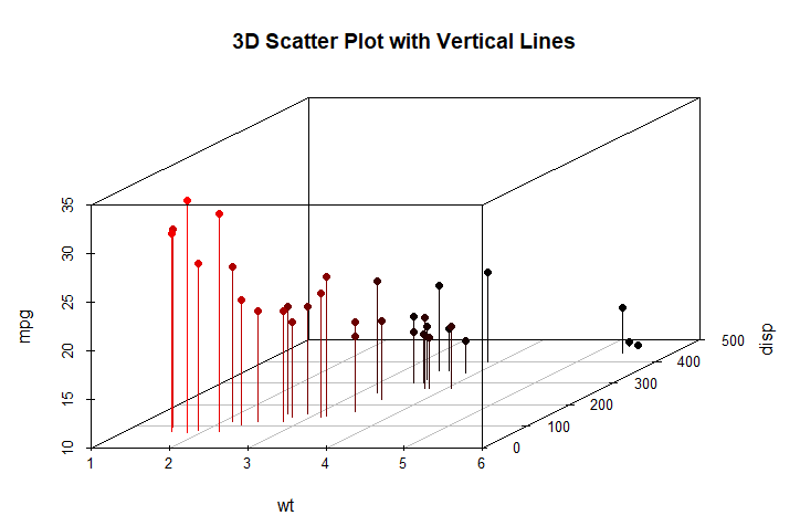
              main="Basic 3D Scatter Plot")

scatterplot3d(wt, disp, mpg,

              pch=16,

              highlight.3d=TRUE,

              type="h",

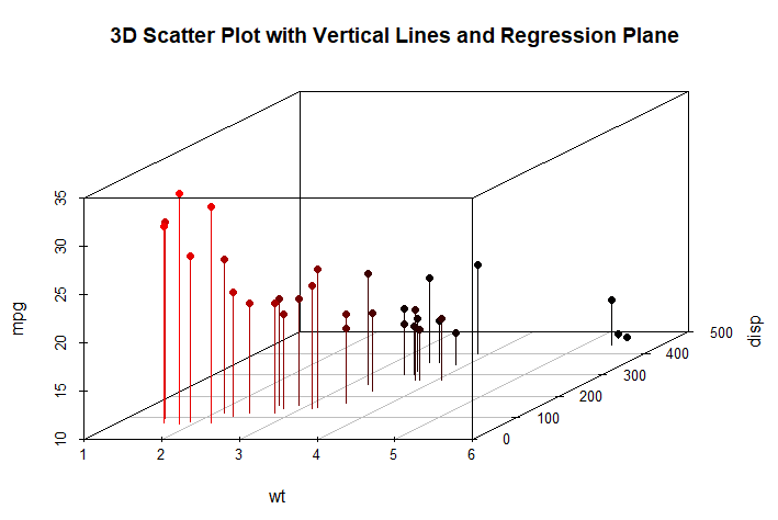
              main="3D Scatter Plot with Vertical Lines")

s3d <-scatterplot3d(wt, disp, mpg,

                    pch=16,

                    highlight.3d=TRUE,

                    type="h",

                    main="3D Scatter Plot with Vertical Lines and Regression Plane")

fit <- lm(mpg ~ wt+disp)

s3d$plane3d(fit)

detach(mtcars)

# spinning 3D plot

library(rgl)

attach(mtcars)

plot3d(wt, disp, mpg, col="red", size=5)

# alternative

library(car)

with(mtcars,

     scatter3d(wt, disp, mpg))

# bubble plots

attach(mtcars)

r <- sqrt(disp/pi)

symbols(wt, mpg, circle=r, inches=0.30,

        fg="white", bg="lightblue",

        main="Bubble Plot with point size proportional to displacement",

        ylab="Miles Per Gallon",

        xlab="Weight of Car (lbs/1000)")

text(wt, mpg, rownames(mtcars), cex=0.6)

detach(mtcars)

# Listing 11.2 - Creating side by side scatter and line plots

opar <- par(no.readonly=TRUE)

par(mfrow=c(1,2))

t1 <- subset(Orange, Tree==1)

plot(t1$age, t1$circumference,

     xlab="Age (days)",

     ylab="Circumference (mm)",

     main="Orange Tree 1 Growth")

plot(t1$age, t1$circumference,

     xlab="Age (days)",

     ylab="Circumference (mm)",

     main="Orange Tree 1 Growth",

     type="b")

par(opar)

# Listing 11.3 - Line chart displaying the growth of 5 Orange trees over time

Orange$Tree <- as.numeric(Orange$Tree)

ntrees <- max(Orange$Tree)

xrange <- range(Orange$age)

yrange <- range(Orange$circumference)

plot(xrange, yrange,

     type="n",

     xlab="Age (days)",

     ylab="Circumference (mm)"

)

colors <- rainbow(ntrees)

linetype <- c(1:ntrees)

plotchar <- seq(18, 18+ntrees, 1)

for (i in 1:ntrees) {

  tree <- subset(Orange, Tree==i)

  lines(tree$age, tree$circumference,

        type="b",

        lwd=2,

        lty=linetype[i],

        col=colors[i],

        pch=plotchar[i]

  )

}

title("Tree Growth", "example of line plot")

legend(xrange[1], yrange[2],

       1:ntrees,

       cex=0.8,

       col=colors,

       pch=plotchar,

       lty=linetype,

       title="Tree"

)                    

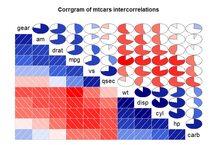
# Correlograms

options(digits=2)

cor(mtcars)

library(corrgram)

corrgram(mtcars, order=TRUE, lower.panel=panel.shade,

         upper.panel=panel.pie, text.panel=panel.txt,

         main="Corrgram of mtcars intercorrelations")

corrgram(mtcars, order=TRUE, lower.panel=panel.ellipse,

         upper.panel=panel.pts, text.panel=panel.txt,

         diag.panel=panel.minmax,

         main="Corrgram of mtcars data using scatter plots

and ellipses")

cols <- colorRampPalette(c("darkgoldenrod4", "burlywood1",

                           "darkkhaki", "darkgreen"))

corrgram(mtcars, order=TRUE, col.regions=cols,

         lower.panel=panel.shade,

         upper.panel=panel.conf, text.panel=panel.txt,

         main="A Corrgram (or Horse) of a Different Color")

# Mosaic Plots

ftable(Titanic)

library(vcd)

mosaic(Titanic, shade=TRUE, legend=TRUE)

library(vcd)

mosaic(~Class+Sex+Age+Survived, data=Titanic, shade=TRUE, legend=TRUE)

# type= options in the plot() and lines() functions

x <- c(1:5)

y <- c(1:5)

par(mfrow=c(2,4))

types <- c("p", "l", "o", "b", "c", "s", "S", "h")

for (i in types){

  plottitle <- paste("type=", i)

  plot(x,y,type=i, col="red", lwd=2, cex=1, main=plottitle)

}