课程一(Neural Networks and Deep Learning)总结—

Deep L-layer neural network

1 - General methodology

As usual you will follow the Deep Learning methodology to build the model:

1). Initialize parameters / Define hyperparameters

2). Loop for num_iterations:

a. Forward propagation

b. Compute cost function

c. Backward propagation

d. Update parameters (using parameters, and grads from backprop)

3). Use trained parameters to predict labels

2 - Architecture of your model

You will build two different models to distinguish cat images from non-cat images.

A 2-layer neural network
An L-layer deep neural network

2.1 - 2-layer neural network

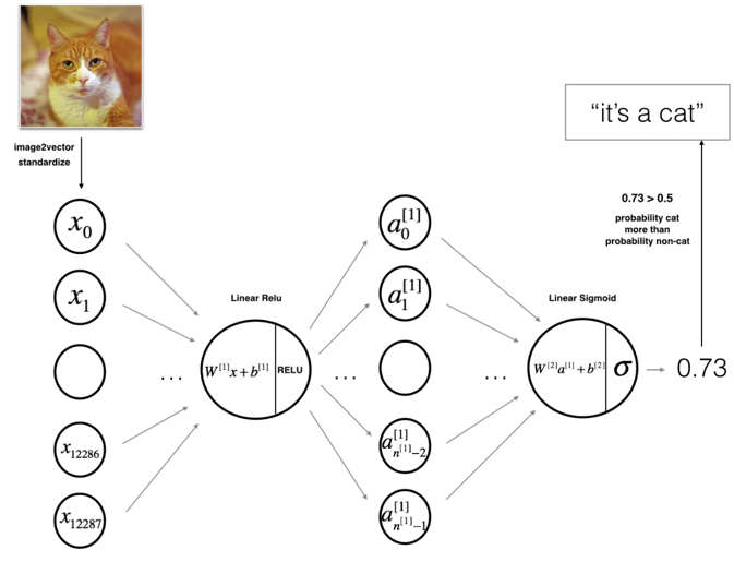
Figure 1: 2-layer neural network.
The model can be summarized as: INPUT -> LINEAR -> RELU
-> LINEAR -> SIGMOID -> OUTPUT.

Detailed Architecture of figure 2:

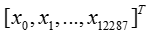
The input is a (64,64,3) image which is flattened to a vector of size (12288,1).
The corresponding vectoris then multiplied by the weight matrix of size
You then add a bias term and take its relu to get the following vector:
You then repeat the same process.You multiply the resulting vector by and add your intercept (bias).
Finally, you take the sigmoid of the result. If it is greater than 0.5, you classify it to be a cat.

2.2 - L-layer deep neural network

Figure 2: L-layer neural network.
The model can be summarized as: [LINEAR -> RELU] × (L-1)
-> LINEAR -> SIGMOID

Detailed Architecture of figure 3:

The input is a (64,64,3) image which is flattened to a vector of size (12288,1).The corresponding vector is then multiplied by the weight matrixand then you add the intercept .The result is called the linear unit.
Next, you take the relu of the linear unit. This process could be repeated several times for each,depending on the model architecture.
Finally, you take the sigmoid of the final linear unit. If it is greater than 0.5, you classify it to be a cat.

3 - Two-layer neural network

Question: Use the helper functions you have implemented to build a 2-layer neural network with the following structure: LINEAR -> RELU -> LINEAR -> SIGMOID. The functions you may need and their inputs are:

def initialize_parameters(n_x, n_h, n_y):

    ...

    return parameters

def linear_activation_forward(A_prev, W, b, activation):

    ...

    return A, cache

def compute_cost(AL, Y):

    ...

    return cost

def linear_activation_backward(dA, cache, activation):

    ...

    return dA_prev, dW, db

def update_parameters(parameters, grads, learning_rate):

    ...

return parameters

def predict(train_x, train_y, parameters)：

    ...

    return Accuracy

3.1 - initialize_parameters(n_x, n_h, n_y)

Create and initialize the parameters of the 2-layer neural network.

Instructions:

The model's structure is: LINEAR -> RELU -> LINEAR -> SIGMOID.
Use random initialization for the weight matrices. Use np.random.randn(shape)*0.01 with the correct shape.
Use zero initialization for the biases. Use np.zeros(shape).

# GRADED FUNCTION: initialize_parameters

def initialize_parameters(n_x, n_h, n_y):

    """

    Argument:

    n_x -- size of the input layer

    n_h -- size of the hidden layer

    n_y -- size of the output layer

    Returns:

    parameters -- python dictionary containing your parameters:

                    W1 -- weight matrix of shape (n_h, n_x)

                    b1 -- bias vector of shape (n_h, 1)

                    W2 -- weight matrix of shape (n_y, n_h)

                    b2 -- bias vector of shape (n_y, 1)

    """

    np.random.seed(1)

    ### START CODE HERE ### (≈ 4 lines of code)

    W1 = np.random.randn(n_h, n_x)*0.01

    b1 = np.zeros((n_h, 1))

    W2 = np.random.randn(n_y, n_h)*0.01

    b2 = np.zeros((n_y, 1))

    ### END CODE HERE ###

    assert(W1.shape == (n_h, n_x))

    assert(b1.shape == (n_h, 1))

    assert(W2.shape == (n_y, n_h))

    assert(b2.shape == (n_y, 1))

    parameters = {"W1": W1,

                  "b1": b1,

                  "W2": W2,

                  "b2": b2}

return parameters

3.2 - linear_activation_forward(A_prev, W, b, activation)

# GRADED FUNCTION: linear_activation_forward

def linear_activation_forward(A_prev, W, b, activation):

    """

    Implement the forward propagation for the LINEAR->ACTIVATION layer

    Arguments:

    A_prev -- activations from previous layer (or input data): (size of previous layer, number of examples)

    W -- weights matrix: numpy array of shape (size of current layer, size of previous layer)

    b -- bias vector, numpy array of shape (size of the current layer, 1)

    activation -- the activation to be used in this layer, stored as a text string: "sigmoid" or "relu"

    Returns:

    A -- the output of the activation function, also called the post-activation value（后面的值）

    cache -- a python dictionary containing "linear_cache" and "activation_cache";

             stored for computing the backward pass efficiently

    """

    if activation == "sigmoid":

        # Inputs: "A_prev, W, b". Outputs: "A, activation_cache".

        ### START CODE HERE ### (≈ 2 lines of code)

        Z, linear_cache =  linear_forward(A_prev, W, b)   # linear_cache （A_prev，W,b）

        A, activation_cache = sigmoid(Z)                  # activation_cache (Z)

        ### END CODE HERE ###

    elif activation == "relu":

        # Inputs: "A_prev, W, b". Outputs: "A, activation_cache".

        ### START CODE HERE ### (≈ 2 lines of code)

        Z, linear_cache =linear_forward(A_prev, W, b)   # linear_cache （A_prev，W,b）

        A, activation_cache = relu(Z)                 # activation_cache (Z)

        ### END CODE HERE ### 

    assert (A.shape == (W.shape[0], A_prev.shape[1]))

    cache = (linear_cache, activation_cache)   # cache (A_prev,W,b,Z)

    return A, cache

3.3 - compute_cost(AL, Y)

Compute the cross-entropy cost J, using the following formula:

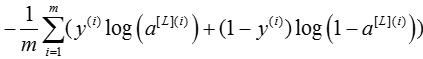
# GRADED FUNCTION: compute_cost

def compute_cost(AL, Y):

    """

    Implement the cost function defined by equation (7).

    Arguments:

    AL -- probability vector corresponding to your label predictions, shape (1, number of examples)

    Y -- true "label" vector (for example: containing 0 if non-cat, 1 if cat), shape (1, number of examples)

    Returns:

    cost -- cross-entropy cost

    """

    m = Y.shape[1]

    # Compute loss from aL and y.

    ### START CODE HERE ### (≈ 1 lines of code)

    cost = - (1/m)*(np.dot(Y, np.log(AL).T) + np.dot(1 - Y, np.log(1-AL).T))

    ### END CODE HERE ###

    cost = np.squeeze(cost)      # To make sure your cost's shape is what we expect (e.g. this turns [[17]] into 17).

    assert(cost.shape == ())

    return cost

3.4 - linear_activation_backward(dA, cache, activation)

# GRADED FUNCTION: linear_activation_backward

def linear_activation_backward(dA, cache, activation):

    """

    Implement the backward propagation for the LINEAR->ACTIVATION layer.

    Arguments:

    dA -- post-activation gradient for current layer l

    cache -- tuple of values (linear_cache, activation_cache) we store for computing backward propagation efficiently

    activation -- the activation to be used in this layer, stored as a text string: "sigmoid" or "relu"

    Returns:

    dA_prev -- Gradient of the cost with respect to the activation (of the previous layer l-1), same shape as A_prev

    dW -- Gradient of the cost with respect to W (current layer l), same shape as W

    db -- Gradient of the cost with respect to b (current layer l), same shape as b

    """

    linear_cache, activation_cache = cache

    if activation == "relu":

        ### START CODE HERE ### (≈ 2 lines of code)

        dZ = relu_backward(dA, activation_cache)

        dA_prev, dW, db = linear_backward(dZ, linear_cache)

        ### END CODE HERE ###

    elif activation == "sigmoid":

        ### START CODE HERE ### (≈ 2 lines of code)

        dZ = sigmoid_backward(dA, activation_cache)

        dA_prev, dW, db = linear_backward(dZ, linear_cache)

        ### END CODE HERE ###

    return dA_prev, dW, db

3.5 - update_parameters

# GRADED FUNCTION: update_parameters

def update_parameters(parameters, grads, learning_rate):

    """

    Update parameters using gradient descent

    Arguments:

    parameters -- python dictionary containing your parameters

    grads -- python dictionary containing your gradients, output of L_model_backward

    Returns:

    parameters -- python dictionary containing your updated parameters

                  parameters["W" + str(l)] = ...

                  parameters["b" + str(l)] = ...

    """

    L = len(parameters) // 2 # number of layers in the neural network

    # Update rule for each parameter. Use a for loop.

    ### START CODE HERE ### (≈ 3 lines of code)

    for l in range(1, L+1):   # l=`,2,3,...,L

         parameters["W" + str(l)] = parameters["W" + str(l)] - learning_rate*grads["dW" + str(l)]

         parameters["b" + str(l)] = parameters["b" + str(l)] - learning_rate*grads["db" + str(l)]

    ### END CODE HERE ###

    return parameters

3.6 - predict(train_x, train_y, parameters)

pred_train = predict(train_x, train_y, parameters)

4 - L-layer neural network

Question: Use the helper functions you have implemented previously to build an LL-layer neural network with the following structure: [LINEAR -> RELU]×(L-1) -> LINEAR -> SIGMOID. The functions you may need and their inputs are:

def initialize_parameters_deep(layer_dims):

    ...

    return parameters

def L_model_forward(X, parameters):

    ...

    return AL, caches

def compute_cost(AL, Y):

    ...

    return cost

def L_model_backward(AL, Y, caches):

    ...

    return grads

def update_parameters(parameters, grads, learning_rate):

    ...

    return parameters

In [14]:

def predict(train_x, train_y, parameters)：

    ...

    return Accuracy

4.1 - initialize_parameters_deep(layer_dims)

Implement initialization for an L-layer Neural Network.

Instructions:

The model's structure is [LINEAR -> RELU] × (L-1) -> LINEAR -> SIGMOID. I.e., it has L−1layers using a ReLU activation function followed by an output layer with a sigmoid activation function.
Use random initialization for the weight matrices. Use np.random.rand(shape) * 0.01.
Use zeros initialization for the biases. Use np.zeros(shape).
We will store , the number of units in different layers, in a variable layer_dims. For example, the layer_dims for the "Planar Data classification model" from last week would have been [2,4,1]: There were two inputs, one hidden layer with 4 hidden units, and an output layer with 1 output unit. Thus means W1's shape was (4,2), b1 was (4,1), W2 was (1,4) and b2 was (1,1). Now you will generalize this to LL layers!
Here is the implementation for L=1(one layer neural network). It should inspire you to implement the general case (L-layer neural network).

 if L == 1:

      parameters["W" + str(L)] = np.random.randn(layer_dims[1], layer_dims[0]) * 0.01

      parameters["b" + str(L)] = np.zeros((layer_dims[1], 1))

# GRADED FUNCTION: initialize_parameters_deep

def initialize_parameters_deep(layer_dims):

    """

    Arguments:

    layer_dims -- python array (list) containing the dimensions of each layer in our network

    Returns:

    parameters -- python dictionary containing your parameters "W1", "b1", ..., "WL", "bL":

                    Wl -- weight matrix of shape (layer_dims[l], layer_dims[l-1])

                    bl -- bias vector of shape (layer_dims[l], 1)

    """

    np.random.seed(3)

    parameters = {}

    L = len(layer_dims)            # number of layers in the network

    for l in range(1, L):

        ### START CODE HERE ### (≈ 2 lines of code)

        parameters['W' + str(l)] =  np.random.randn(layer_dims[l], layer_dims[l-1]) * 0.01

        parameters['b' + str(l)] =  np.zeros((layer_dims[l], 1))

        ### END CODE HERE ###

        assert(parameters['W' + str(l)].shape == (layer_dims[l], layer_dims[l-1]))

        assert(parameters['b' + str(l)].shape == (layer_dims[l], 1))

    return parameters

4.2 - L_model_forward(X, parameters)

# GRADED FUNCTION: L_model_forward

def L_model_forward(X, parameters):

    """

    Implement forward propagation for the [LINEAR->RELU]*(L-1)->LINEAR->SIGMOID computation

    Arguments:

    X -- data, numpy array of shape (input size, number of examples)

    parameters -- output of initialize_parameters_deep()

    Returns:

    AL -- last post-activation value

    caches -- list of caches containing:

                every cache of linear_relu_forward() (there are L-1 of them, indexed from 0 to L-2)

                the cache of linear_sigmoid_forward() (there is one, indexed L-1)

    """

    caches = []

    A = X

    L = len(parameters) // 2       # number of layers in the neural network

    # Implement [LINEAR -> RELU]*(L-1). Add "cache" to the "caches" list.

    for l in range(1, L):   #注意range是(1,L),最后的L不算进循环，l实际是从1到 L-1

        A_prev = A

        ### START CODE HERE ### (≈ 2 lines of code)

        A, cache = linear_activation_forward(A_prev, parameters['W'+str(l)], parameters['b'+str(l)], activation = "relu")

        caches.append(cache)

        ### END CODE HERE ###

    # Implement LINEAR -> SIGMOID. Add "cache" to the "caches" list.

    ### START CODE HERE ### (≈ 2 lines of code)

    AL, cache = linear_activation_forward(A, parameters['W'+str(L)], parameters['b'+str(L)], activation = "sigmoid")

    caches.append(cache)

    ### END CODE HERE ###

    assert(AL.shape == (1,X.shape[1]))

    return AL, caches   # caches (A_prev,W,b,Z)

4.3 - compute_cost(AL, Y)

Compute the cross-entropy cost J, using the following formula:

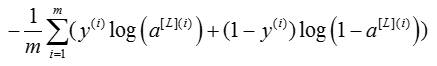
# GRADED FUNCTION: compute_cost

def compute_cost(AL, Y):

    """

    Implement the cost function defined by equation (7).

    Arguments:

    AL -- probability vector corresponding to your label predictions, shape (1, number of examples)

    Y -- true "label" vector (for example: containing 0 if non-cat, 1 if cat), shape (1, number of examples)

    Returns:

    cost -- cross-entropy cost

    """

    m = Y.shape[1]

    # Compute loss from aL and y.

    ### START CODE HERE ### (≈ 1 lines of code)

    cost = - (1/m)*(np.dot(Y, np.log(AL).T) + np.dot(1 - Y, np.log(1-AL).T))

    ### END CODE HERE ###

    cost = np.squeeze(cost)      # To make sure your cost's shape is what we expect (e.g. this turns [[17]] into 17).

    assert(cost.shape == ())

    return cost

4.4 - L_model_backward(AL, Y, caches)

# GRADED FUNCTION: L_model_backward

def L_model_backward(AL, Y, caches):

    """

    Implement the backward propagation for the [LINEAR->RELU] * (L-1) -> LINEAR -> SIGMOID group

    Arguments:

    AL -- probability vector, output of the forward propagation (L_model_forward())

    Y -- true "label" vector (containing 0 if non-cat, 1 if cat)

    caches -- list of caches containing:

                every cache of linear_activation_forward() with "relu" (it's caches[l], for l in range(L-1) i.e l = 0...L-2)

                the cache of linear_activation_forward() with "sigmoid" (it's caches[L-1])

    Returns:

    grads -- A dictionary with the gradients

             grads["dA" + str(l)] = ...

             grads["dW" + str(l)] = ...

             grads["db" + str(l)] = ...

    """

    grads = {}

    L = len(caches) # the number of layers

    m = AL.shape[1]

    Y = Y.reshape(AL.shape) # after this line, Y is the same shape as AL

    # Initializing the backpropagation

    ### START CODE HERE ### (1 line of code)

    dAL = - (np.divide(Y, AL) - np.divide(1 - Y, 1 - AL)) # derivative of cost with respect to AL

    ### END CODE HERE ###

    # Lth layer (SIGMOID -> LINEAR) gradients. Inputs: "AL, Y, caches". Outputs: "grads["dAL"], grads["dWL"], grads["dbL"]

    ### START CODE HERE ### (approx. 2 lines)

    current_cache = caches[L-1]

    grads["dA" + str(L)], grads["dW" + str(L)], grads["db" + str(L)] =linear_activation_backward(dAL, current_cache, activation = "sigmoid")

    ### END CODE HERE ###

    for l in reversed(range(L-1)):  # l=L-2,L-3,...,2,1,0

        # lth layer: (RELU -> LINEAR) gradients.

        # Inputs: "grads["dA" + str(l + 2)], caches". Outputs: "grads["dA" + str(l + 1)] , grads["dW" + str(l + 1)] , grads["db" + str(l + 1)]

        ### START CODE HERE ### (approx. 5 lines)

        current_cache =  caches[l]    # l= L-2,L-1,...,2,1,0   当l=L-2时

        dA_prev_temp, dW_temp, db_temp = linear_activation_backward(grads["dA" + str(l+2)], current_cache, activation = "relu")  # l+2=L

        grads["dA" + str(l + 1)] = dA_prev_temp     #l=L-1

        grads["dW" + str(l + 1)] = dW_temp      #l+1=L-1

        grads["db" + str(l + 1)] = db_temp      #l+1=L-1

        ### END CODE HERE ###

    return grads

4.5 - update_parameters

# GRADED FUNCTION: update_parameters

def update_parameters(parameters, grads, learning_rate):

    """

    Update parameters using gradient descent

    Arguments:

    parameters -- python dictionary containing your parameters

    grads -- python dictionary containing your gradients, output of L_model_backward

    Returns:

    parameters -- python dictionary containing your updated parameters

                  parameters["W" + str(l)] = ...

                  parameters["b" + str(l)] = ...

    """

    L = len(parameters) // 2 # number of layers in the neural network

    # Update rule for each parameter. Use a for loop.

    ### START CODE HERE ### (≈ 3 lines of code)

    for l in range(1, L+1):   # l=`,2,3,...,L

         parameters["W" + str(l)] = parameters["W" + str(l)] - learning_rate*grads["dW" + str(l)]

         parameters["b" + str(l)] = parameters["b" + str(l)] - learning_rate*grads["db" + str(l)]

    ### END CODE HERE ###

    return parameters

4.6 - predict(train_x, train_y, parameters)

pred_train = predict(train_x, train_y, parameters)

pred_test = predict(test_x, test_y, parameters)

【参考】：

[1] https://hub.coursera-notebooks.org/user/rdzflaokljifhqibzgygqq/notebooks/Week%204/Deep%20Neural%20Network%20Application:%20Image%20Classification/Deep%20Neural%20Network%20-%20Application%20v3.ipynb

[2] https://hub.coursera-notebooks.org/user/rdzflaokljifhqibzgygqq/notebooks/Week%204/Building%20your%20Deep%20Neural%20Network%20-%20Step%20by%20Step/Building%20your%20Deep%20Neural%20Network%20-%20Step%20by%20Step%20v5.ipynb

【附录】：

L层神经网络的详细推导，见hezhiyao的github: https://github.com/hezhiyao/Deep-L-layer-neural-network-Notes

巴特西

课程一(Neural Networks and Deep Learning)总结——2、Deep Neural Networks

最新文章

热门文章