机器学习 - 算法 - SVM 支持向量机 Py 实现 / 人脸识别案例
SVM 代码实现展示
相关模块引入
%matplotlib inline

import numpy as np

import matplotlib.pyplot as plt

from scipy import stats

import seaborn as sns;sns.set() # 使用seaborn的默认设置
数据集
这里自己生成一些随机数据
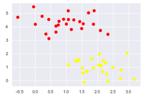
#随机来点数据

from sklearn.datasets.samples_generator import make_blobs

X, y = make_blobs(

    n_samples=50, # 样本点数量

    centers=2,  # 簇堆数量

    random_state=0,  # 随机种子

    cluster_std=0.60  # 簇离散程度

)

plt.scatter(X[:, 0], X[:, 1], c=y, s=50, cmap='autumn')
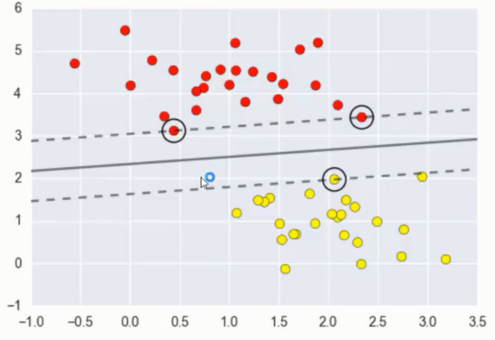
切分数据
xfit = np.linspace(-1, 3.5)

plt.scatter(X[:, 0], X[:, 1], c=y, s=50, cmap='autumn')

plt.plot([0.6], [2.1], 'x', color='red', markeredgewidth=2, markersize=10)

for m, b in [(1, 0.65), (0.5, 1.6), (-0.2, 2.9)]:

    plt.plot(xfit, m * xfit + b, '-k')

plt.xlim(-1, 3.5);
如图所示分开有很多种方式, 看哪种更好呢?

最小化雷区
xfit = np.linspace(-1, 3.5)

plt.scatter(X[:, 0], X[:, 1], c=y, s=50, cmap='autumn')

for m, b, d in [(1, 0.65, 0.33), (0.5, 1.6, 0.55), (-0.2, 2.9, 0.2)]:

    yfit = m * xfit + b

    plt.plot(xfit, yfit, '-k')

    plt.fill_between(xfit, yfit - d, yfit + d, edgecolor='none',

                     color='#AAAAAA', alpha=0.4)

plt.xlim(-1, 3.5);
画出来他的决策边界即可看出宽度

训练一个基本的SVM
from sklearn.svm import SVC # "Support vector classifier"

model = SVC(kernel='linear')

model.fit(X, y)
SVC(C=1.0, cache_size=200, class_weight=None, coef0=0.0,

  decision_function_shape=None, degree=3, gamma='auto', kernel='linear',

  max_iter=-1, probability=False, random_state=None, shrinking=True,

  tol=0.001, verbose=False)
绘图展示
#绘图函数

def plot_svc_decision_function(model, ax=None, plot_support=True):

    """Plot the decision function for a 2D SVC"""

    if ax is None:

        ax = plt.gca()

    xlim = ax.get_xlim()

    ylim = ax.get_ylim()

    # create grid to evaluate model

    x = np.linspace(xlim[0], xlim[1], 30)

    y = np.linspace(ylim[0], ylim[1], 30)

    Y, X = np.meshgrid(y, x)

    xy = np.vstack([X.ravel(), Y.ravel()]).T

    P = model.decision_function(xy).reshape(X.shape)

    # plot decision boundary and margins

    ax.contour(X, Y, P, colors='k',

               levels=[-1, 0, 1], alpha=0.5,

               linestyles=['--', '-', '--'])

    # plot support vectors

    if plot_support:

        ax.scatter(model.support_vectors_[:, 0],

                   model.support_vectors_[:, 1],

                   s=300, linewidth=1, facecolors='none');

    ax.set_xlim(xlim)

    ax.set_ylim(ylim)
plt.scatter(X[:, 0], X[:, 1], c=y, s=50, cmap='autumn')

plot_svc_decision_function(model);
这条线就是我们希望得到的决策边界啦
观察发现有3个点做了特殊的标记,它们恰好都是边界上的点
它们就是我们的support vectors(支持向量)
在Scikit-Learn中, 它们存储在 support_vectors_ 属性中
model.support_vectors_
array([[0.44359863, 3.11530945],

       [2.33812285, 3.43116792],

       [2.06156753, 1.96918596]])
观察可以发现,只需要支持向量我们就可以把模型构建出来
样本密闭程度不同对决策影响
接下来我们尝试一下,用不同多的数据点,看看效果会不会发生变化
分别使用60个和120个数据点
def plot_svm(N=10, ax=None):

    X, y = make_blobs(n_samples=200, centers=2,

                      random_state=0, cluster_std=0.60)

    X = X[:N]

    y = y[:N]

    model = SVC(kernel='linear', C=1E10)

    model.fit(X, y)

    ax = ax or plt.gca()

    ax.scatter(X[:, 0], X[:, 1], c=y, s=50, cmap='autumn')

    ax.set_xlim(-1, 4)

    ax.set_ylim(-1, 6)

    plot_svc_decision_function(model, ax)

fig, ax = plt.subplots(1, 2, figsize=(16, 6))

fig.subplots_adjust(left=0.0625, right=0.95, wspace=0.1)

for axi, N in zip(ax, [60, 120]):

    plot_svm(N, axi)

    axi.set_title('N = {0}'.format(N))
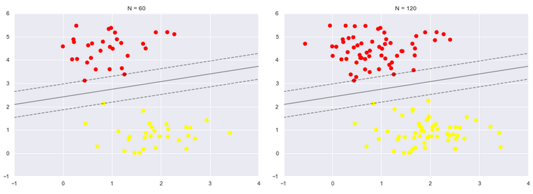
左边是60个点的结果,右边的是120个点的结果
观察发现,只要支持向量没变,其他的数据怎么加无所谓!
引入核函数的 SVM
对比线性核展示
首先我们先用线性的核来看一下在下面这样比较难的数据集上还能分了吗?
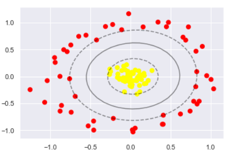
from sklearn.datasets.samples_generator import make_circles
X, y = make_circles(100, factor=.1, noise=.1)# 二维圆形数据 factor 内外圆比例 (0,1)clf = SVC(kernel='linear').fit(X, y) plt.scatter(X[:, 0], X[:, 1], c=y, s=50, cmap='autumn')
plot_svc_decision_function(clf, plot_support=False);
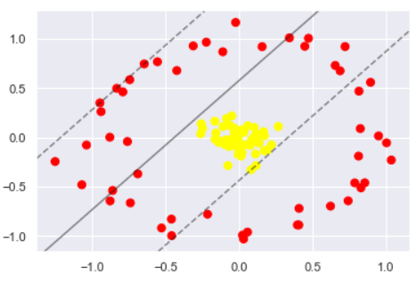
可以看出完全分不开的
核变换空间展示原理
相当于将二维的数据引入三维, 然后在新加入的维度中提升位置, 然后在切, 即可以分开了
#加入了新的维度r
from mpl_toolkits import mplot3d
r = np.exp(-(X ** 2).sum(1))
def plot_3D(elev=30, azim=30, X=X, y=y):
ax = plt.subplot(projection='3d')
ax.scatter3D(X[:, 0], X[:, 1], r, c=y, s=50, cmap='autumn')
ax.view_init(elev=elev, azim=azim)# 设置3D视图的角度 一般都为45
ax.set_xlabel('x')
ax.set_ylabel('y')
ax.set_zlabel('r') plot_3D(elev=45, azim=45, X=X, y=y)

实际操作 - 引入径向基函数
#加入径向基函数

clf = SVC(kernel='rbf', C=1E6)

clf.fit(X, y)
SVC(C=1000000.0, cache_size=200, class_weight=None, coef0=0.0,

  decision_function_shape=None, degree=3, gamma='auto', kernel='rbf',

  max_iter=-1, probability=False, random_state=None, shrinking=True,

  tol=0.001, verbose=False)
plt.scatter(X[:, 0], X[:, 1], c=y, s=50, cmap='autumn')

plot_svc_decision_function(clf)

plt.scatter(clf.support_vectors_[:, 0], clf.support_vectors_[:, 1],

            s=300, lw=1, facecolors='none');
调节 SVM 参数 - Soft Margin 问题
C 参数调整
软间隔设置的 C 参数调整
当C趋近于无穷大时:意味着分类严格不能有错误
当C趋近于很小的时:意味着可以有更大的错误容忍
这里将数据的离散程度稍微大一点, 让决策边界的难度更高一些
X, y = make_blobs(n_samples=100, centers=2,

                  random_state=0, cluster_std=0.8)

plt.scatter(X[:, 0], X[:, 1], c=y, s=50, cmap='autumn');
X, y = make_blobs(n_samples=100, centers=2,

                  random_state=0, cluster_std=0.8)

fig, ax = plt.subplots(1, 2, figsize=(16, 6))

fig.subplots_adjust(left=0.0625, right=0.95, wspace=0.1)

for axi, C in zip(ax, [10.0, 0.1]):

    model = SVC(kernel='linear', C=C).fit(X, y)

    axi.scatter(X[:, 0], X[:, 1], c=y, s=50, cmap='autumn')

    plot_svc_decision_function(model, axi)

    axi.scatter(model.support_vectors_[:, 0],

                model.support_vectors_[:, 1],

                s=300, lw=1, facecolors='none');

    axi.set_title('C = {0:.1f}'.format(C), size=14)
设定 C 为 10 和 0.1 的时候的对比, 可以看出比较严格的时候, 泛化能力较差

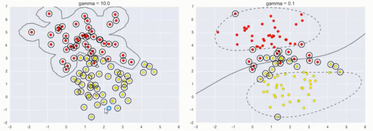
伽玛值参数调整
伽玛值在这里的意义是限制你模型的映射维度, 伽玛值这个参数是只有 SVM 中才有的
越大映射维度越高, 越小则维度越小
维度影响到模型的复杂程度, 越不复杂的模型得出的结果也就越平稳
X, y = make_blobs(n_samples=100, centers=2,

                  random_state=0, cluster_std=1.1)

fig, ax = plt.subplots(1, 2, figsize=(16, 6))

fig.subplots_adjust(left=0.0625, right=0.95, wspace=0.1)

for axi, gamma in zip(ax, [10.0, 0.1]):

    model = SVC(kernel='rbf', gamma=gamma).fit(X, y)

    axi.scatter(X[:, 0], X[:, 1], c=y, s=50, cmap='autumn')

    plot_svc_decision_function(model, axi)

    axi.scatter(model.support_vectors_[:, 0],

                model.support_vectors_[:, 1],

                s=300, lw=1, facecolors='none');

    axi.set_title('gamma = {0:.1f}'.format(gamma), size=14)
取值依旧是 10 和 0.1
可以看出 10 的时候的决策边界相当的负责且严格
而 0.1 的时候更加柔和平稳, 但是也分错了很多数据点
应用人脸识别实例
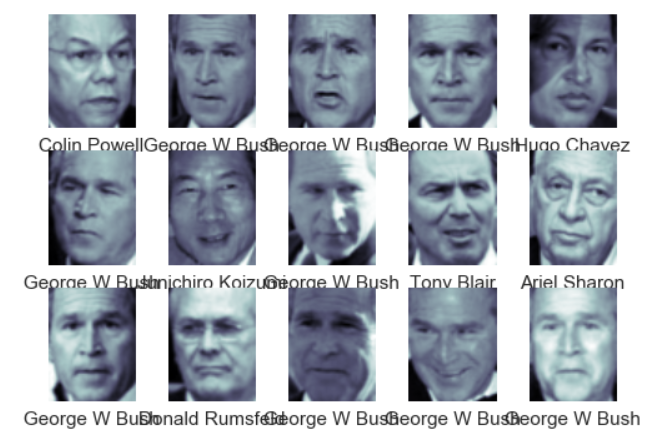
数据集
还是个分类任务, 判定人脸是谁, 数据集需要下载, 大概大小在 200M 左右
from sklearn.datasets import fetch_lfw_people

faces = fetch_lfw_people(min_faces_per_person=60)

print(faces.target_names)

print(faces.images.shape)
首先过筛了一遍数据, 少于 60 个的都过滤掉
['Ariel Sharon' 'Colin Powell' 'Donald Rumsfeld' 'George W Bush'

 'Gerhard Schroeder' 'Hugo Chavez' 'Junichiro Koizumi' 'Tony Blair']

(1348, 62, 47)
展示数据集内容
fig, ax = plt.subplots(3, 5)

for i, axi in enumerate(ax.flat):

    axi.imshow(faces.images[i], cmap='bone')

    axi.set(xticks=[], yticks=[],

            xlabel=faces.target_names[faces.target[i]])
每个图的大小是 [62×47]
创建 SVM 模型
在这里我们就把每一个像素点当成了一个特征,但是这样特征太多了,用 PCA 降维后创建模型
from sklearn.svm import SVC

#from sklearn.decomposition import RandomizedPCA

from sklearn.decomposition import PCA

from sklearn.pipeline import make_pipeline

pca = PCA(n_components=150, whiten=True, random_state=42)

svc = SVC(kernel='rbf', class_weight='balanced')

model = make_pipeline(pca, svc)
切分训练 / 测试集
from sklearn.model_selection import train_test_split

Xtrain, Xtest, ytrain, ytest = train_test_split(faces.data, faces.target,

                                                random_state=40)
选择最佳参数
使用 grid search cross-validation来选择参数
from sklearn.model_selection import GridSearchCV

param_grid = {'svc__C': [1, 5, 10],

              'svc__gamma': [0.0001, 0.0005, 0.001]}

grid = GridSearchCV(model, param_grid)

%time grid.fit(Xtrain, ytrain)

print(grid.best_params_)
Wall time: 51.5 s

{'svc__C': 5, 'svc__gamma': 0.001}
选出的 C = 5 , gamma = 0.001
预测
model = grid.best_estimator_

yfit = model.predict(Xtest)

yfit.shape
(337,)
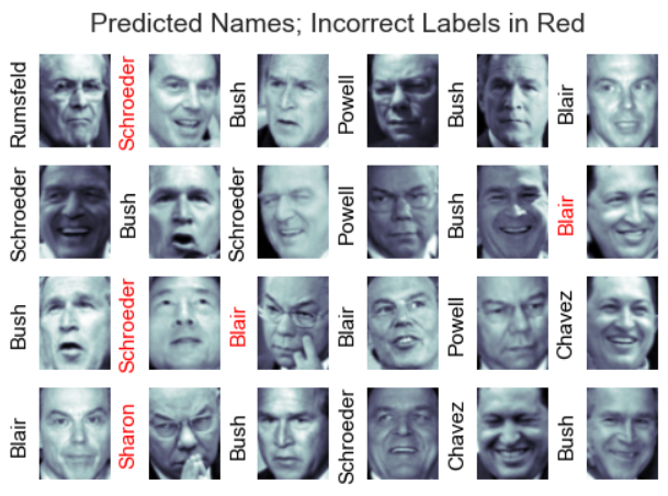
画图展示
预测成功的就用黑色, 不成功用 红色表示
fig, ax = plt.subplots(4, 6)

for i, axi in enumerate(ax.flat):

    axi.imshow(Xtest[i].reshape(62, 47), cmap='bone')

    axi.set(xticks=[], yticks=[])

    axi.set_ylabel(faces.target_names[yfit[i]].split()[-1],

                   color='black' if yfit[i] == ytest[i] else 'red')

fig.suptitle('Predicted Names; Incorrect Labels in Red', size=14);
个人结果展示
详细的对每个人的预测结果展示
from sklearn.metrics import classification_report

print(classification_report(ytest, yfit,

                            target_names=faces.target_names))
                  precision    recall  f1-score   support

     Ariel Sharon       0.50      0.50      0.50        16

     Colin Powell       0.69      0.81      0.75        54

  Donald Rumsfeld       0.83      0.85      0.84        34

    George W Bush       0.94      0.88      0.91       136

Gerhard Schroeder       0.72      0.85      0.78        27

      Hugo Chavez       0.81      0.72      0.76        18

Junichiro Koizumi       0.87      0.87      0.87        15

       Tony Blair       0.85      0.76      0.80        37

      avg / total       0.83      0.82      0.82       337
- 精度(precision) = 正确预测的个数(TP)/被预测正确的个数(TP+FP)
- 召回率(recall)=正确预测的个数(TP)/预测个数(TP+FN)
- F1 = 2精度召回率/(精度+召回率)
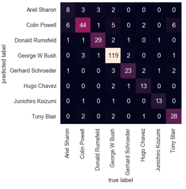
混淆矩阵展示
通过混淆矩阵可以看出那些人容易被认错成什么人
from sklearn.metrics import confusion_matrix

mat = confusion_matrix(ytest, yfit)

sns.heatmap(mat.T, square=True, annot=True, fmt='d', cbar=False,

            xticklabels=faces.target_names,

            yticklabels=faces.target_names)

plt.xlabel('true label')

plt.ylabel('predicted label');
最新文章
- 【总结】虚拟机VirtualBox各种使用技巧
- iOS开发---集成百度地图,位置偏移问题
- myeclipse10安装findbugs
- ZOJ 2588 Burning Bridges (tarjan求割边)
- css斜线
- javascript中document对象的属性和方法
- javascript权威指南学习笔记3
- gridview两列数据的互换
- Github Pages 搭建HEXO主题个人博客
- C#版的 Escape() 和 Unescape()
- TensorFlow卷积层-函数
- Mosquitto --topic
- gith命令行使用之上传和删除
- Wow! Such Doge! HDU - 4847(虽然是道水题 但很有必要记一下)
- C#资源释放及Dispose、Close和析构方法
- Java的枚举类型
- SQL学习笔记之SQL中INNER、LEFT、RIGHT JOIN的区别和用法详解
- 373. Partition Array by Odd and Even【LintCode java】
- 通过javascript进行UTF-8编码
- 题解 P1436 【棋盘分割】
热门文章
- Windows Server 2008更改SID
- 运维开发笔记整理-使用Django编写helloworld
- flask中使用ajax 处理前端请求,每隔一段时间请求不通的接口,结果展示同一页面
- 微服务学习及.net core入门教程
- Python 高级
- 专为简化 C 开发而设计的编程语言 Trad
- Tomcat报错:Java.long.nullpointerException,详细是resp.getwriter.write报错
- idea在src/main/java下新建包后项目中只显示src/main,后面的东西不显示,但在本地磁盘中是存在的
- java获取远程服务器应用程序服务状态
- PostgreSQL 数据目录结构