% Analog Signal

Dt = 0.00005; t = -0.005:Dt:0.005; xa = exp(-1000*abs(t));

% Discrete-time Signal

Ts = 0.0002; n = -25:1:25; x = exp(-1000*abs(n*Ts));

% Discrete-time Fourier Transform

%Wmax = 2*pi*2000;

K = 500; k = 0:1:K; w = pi*k/K;                 % index array k for frequencies

X = x * exp(-j*n'*w); 

magX  = abs(X);  angX  = angle(X);  realX  = real(X);  imagX  = imag(X);

%% --------------------------------------------------------------------

%%              START X's  mag ang real imag

%% --------------------------------------------------------------------

figure('NumberTitle', 'off', 'Name', 'Example3.19a X its mag ang real imag');

set(gcf,'Color','white');

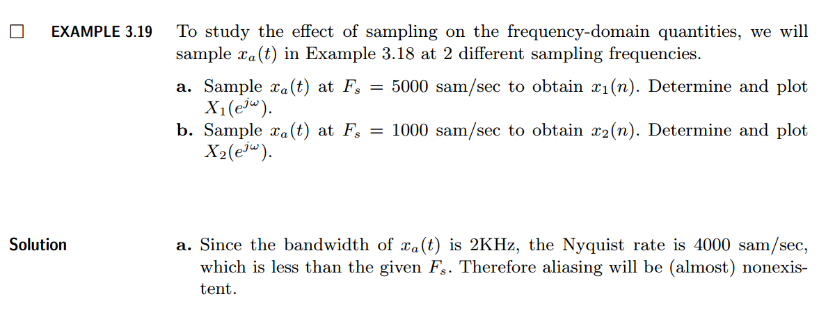
subplot(2,2,1); plot(w/pi,magX); grid on;  %axis([0,1,0,1.5]);

title('Magnitude Response');

xlabel('frequency in \pi units'); ylabel('Magnitude  |X|');

subplot(2,2,3); plot(w/pi, angX/pi); grid on; % axis([-1,1,-1,1]);

title('Phase Response');

xlabel('frequency in \pi units'); ylabel('Radians/\pi');

subplot('2,2,2'); plot(w/pi, realX); grid on;

title('Real Part');

xlabel('frequency in \pi units'); ylabel('Real');

subplot('2,2,4'); plot(w/pi, imagX); grid on;

title('Imaginary Part');

xlabel('frequency in \pi units'); ylabel('Imaginary');

%% -------------------------------------------------------------------

%%             END X's  mag ang real imag

%% -------------------------------------------------------------------

X = real(X);

w = [-fliplr(w), w(2:K+1)];                     % Omega from -Wmax to Wmax

X = [fliplr(X), X(2:K+1)];                      % X over -Wmax to Wmax interval

%% --------------------------------------------------------------------

%%

%% --------------------------------------------------------------------

figure('NumberTitle', 'off', 'Name', '<<DSP MATLAB>> Example3.19a');

set(gcf,'Color','white');

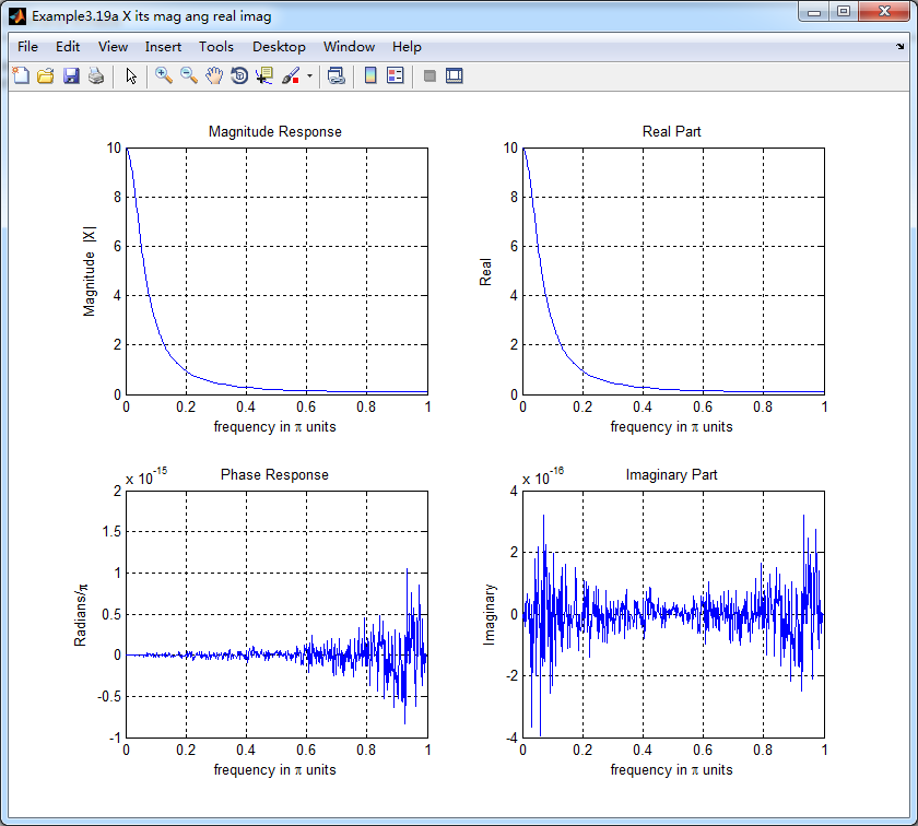
subplot(2,1,1); plot(t*1000,xa); grid on;  %axis([0,1,0,1.5]);

title('Discrete Signal');

xlabel('t in msec units.'); ylabel('x1(n)'); hold on;

stem(n*Ts*1000,x); gtext('Ts=0.2 msec'); hold off;

subplot(2,1,2); plot(w/pi, X); grid on; % axis([-1,1,-1,1]);

title('Discrete-time Fourier Transform');

xlabel('frequency in \pi units'); ylabel('X1(w)');

%% -------------------------------------------------------------------

%%

%% -------------------------------------------------------------------

% Analog Signal

Dt = 0.00005; t = -0.005:Dt:0.005; xa = exp(-1000*abs(t));

% Discrete-time Signal

%Ts = 0.0002; n = -25:1:25; x = exp(-1000*abs(n*Ts));

Ts = 0.001; n = -5:1:5; x = exp(-1000*abs(n*Ts));

% Discrete-time Fourier Transform

%Wmax = 2*pi*2000;

K = 500; k = 0:1:K; w = pi*k/K;                 % index array k for frequencies

X = x * exp(-j*n'*w); 

magX  = abs(X);  angX  = angle(X);  realX  = real(X);  imagX  = imag(X);

%% --------------------------------------------------------------------

%%              START X's  mag ang real imag

%% --------------------------------------------------------------------

figure('NumberTitle', 'off', 'Name', 'Example3.19b X its mag ang real imag');

set(gcf,'Color','white');

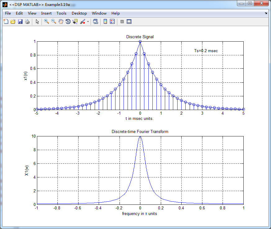
subplot(2,2,1); plot(w/pi,magX); grid on;  %axis([0,1,0,1.5]);

title('Magnitude Response');

xlabel('frequency in \pi units'); ylabel('Magnitude  |X|');

subplot(2,2,3); plot(w/pi, angX/pi); grid on; % axis([-1,1,-1,1]);

title('Phase Response');

xlabel('frequency in \pi units'); ylabel('Radians/\pi');

subplot('2,2,2'); plot(w/pi, realX); grid on;

title('Real Part');

xlabel('frequency in \pi units'); ylabel('Real');

subplot('2,2,4'); plot(w/pi, imagX); grid on;

title('Imaginary Part');

xlabel('frequency in \pi units'); ylabel('Imaginary');

%% -------------------------------------------------------------------

%%             END X's  mag ang real imag

%% -------------------------------------------------------------------

X = real(X);

w = [-fliplr(w), w(2:K+1)];                     % Omega from -Wmax to Wmax

X = [fliplr(X), X(2:K+1)];                      % X over -Wmax to Wmax interval

%% --------------------------------------------------------------------

%%

%% --------------------------------------------------------------------

figure('NumberTitle', 'off', 'Name', '<<DSP MATLAB>> Example3.19b');

set(gcf,'Color','white');

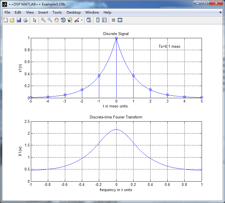
subplot(2,1,1); plot(t*1000,xa); grid on;  %axis([0,1,0,1.5]);

title('Discrete Signal');

xlabel('t in msec units.'); ylabel('x1(n)'); hold on;

stem(n*Ts*1000,x); gtext('Ts=0.1 msec'); hold off;

subplot(2,1,2); plot(w/pi, X); grid on; % axis([-1,1,-1,1]);

title('Discrete-time Fourier Transform');

xlabel('frequency in \pi units'); ylabel('X1(w)');

%% -------------------------------------------------------------------

%%

%% -------------------------------------------------------------------