ELK Stack总结
ELK Stack
本文基于ELK 6.0,主要针对Elasticsearch和Kibana。
介绍
Elasticsearch is a realtime, distributed search and analytics engine that is horizontally scalable and capable of solving a wide variety of use cases.
优势
- Schemaless, document-oriented:存储JSON documents,更加灵活(不规定每条数据的必须具备哪些列)
- Searching:全文text检索,日期、数字、地理位置、IP地址等都可以。
- Analytics:尤其是明细数据
- Rich client library support and the REST API Easy to operate and easy to scale 部署简单、外部依赖少
- Near real time, Lightning fast, Fault tolerant
缺点:资源更多,需要更多机器。在数据量大时聚合统计方面查询延迟与并发不如Druid。
组成
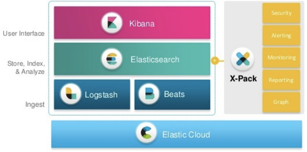
Elasticsearch:作为核心,存储所有数据,提供搜索和分析。
Logstash:集中数据,包括日志、指标等(类似flume)。集中时可以对数据进行各种转换,定位为ETL引擎。
Logstash的Shipper、Broker、Indexer分别和Flume的Source、Channel、Sink各自对应!只不过是Logstash集成了,Broker可以不需要,而Flume需要单独配置,且缺一不可。总体来说Flume的配置比较繁琐,偏向数据传输,Logstash更简单且功能也更多,如解析预处理。
Kibana:ES的可视化工具。
Elasticsearch
概念1(基础)
Elasticsearch是文件导向型存储,JSON文件是第一公民。
索引:含有相同属性的文档集合(小写不含下划线),相当于database。分结构化和非结构化
类型:索引可以定义一个或多个类型,文档必须属于一个类型,相当于table
文档:可以被索引的基本数据单位,相当于record。
在6.0后,索引只能有一个类型。
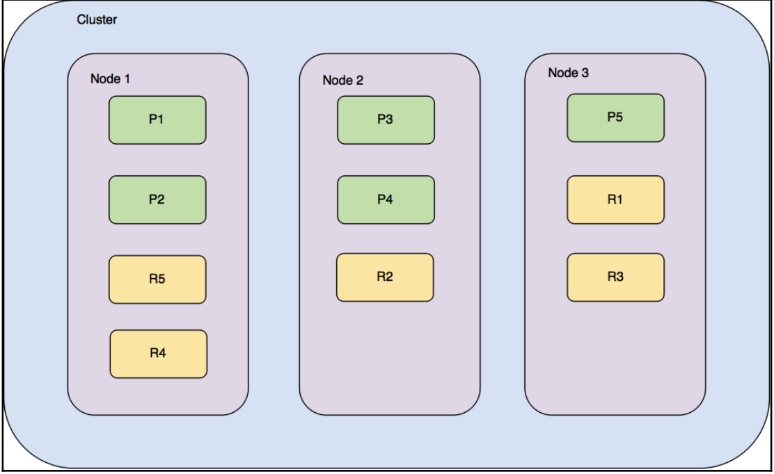
分片:每个索引都有很多个分片,每个分片是一个Lucene索引。只能创建索引时指定数量,默认为5。
备份:拷贝一份分片就完成了分片的备份
数据类型
text data, numbers, booleans, binary objects, arrays, objects, nested types, geo-points, geo-shapes, and many other specialized datatypes such as IPv4 and IPv6 addresses
6.0引入scaled_float,其存储价格数据效率高,例如10.05在内部实际上是1005的integer。
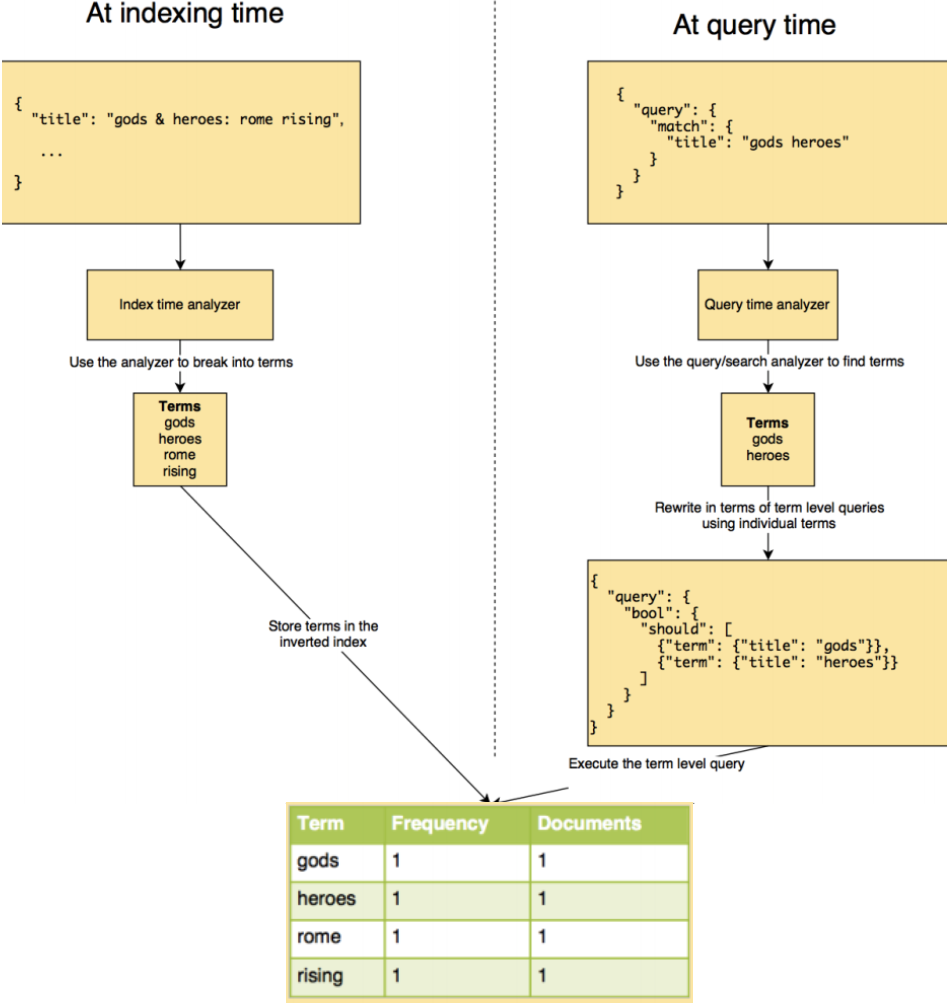
elasticsearch采用倒排索引的数据结构,分为Term,Frequency和Documents (Postings)三列。其中term为词,Documents列也可能存储改词在文本中的位置。默认elasticsearch会对所有field创建倒排索引。当插入document时,elasticsearch就会解析这个document所有的filed,并添加到倒排索引中。
CRUD基本用法
Restful API基本格式:http://<ip>:<port>/<索引>/<类型>/<文档id>
常用的四种请求方式:GET、PUT、POST、DELETE
PUT: 创建索引和文档增加
POST: 文档增加、查询索引和文档修改
GET: 查询文档
DELETE: 删除文档和删除索引
如果不想自己设置文档id,那就需要用post而不是put
创建结构化索引
如果不创建而直接put来插入数据,elasticsearch会自动创建索引和类型,但一些默认设置可能不会符合预期。所以这里就直接放手动创建index的例子了。另外,如果put的数据包含新的field,elasticsearch也会自动创建新的field。
在postman中put下面json到localhost:9200/index_name
例子1,下面的json会创建索引和类型(名为man)

{

	"settings": {

		"number_of_shards": 3,

		"number_of_replicas": 1

	},

	"mappings": {

		"man": { // 类型

			"properties": {

				"country": {

					"type": "keyword"

				},

				"age": {

					"type": "integer"

				},

				"date": {

					"type": "date",

					"format": "yyyy-MM-dd HH:mm:ss || yyyy-MM-dd||epoch_millis"

				}

			}

		}

	}

}

// 添加新类型。下面假设已经创建了catalog index,那么执行下面语句就会新增一个category类型。如果第二次执行下面代码,换成不同的field,那么就是添加新field

PUT /catalog/_mapping/category

{

  "properties": {

    "name": {

      "type": "text"

    }

  }

}

例子2

{

  "settings": {

    "number_of_replicas": 0,

    "number_of_shards": 5, // 一般将分片限制在10~20G

    "index.store.type": "niofs" ,// 性能更好

    "index.query.default_field": "title", // 默认查询字段

    "index.unassigned.node_left.delayed_timeout": "5m" // 当某个节点挂掉时,不马上回复分片

     "analysis": { // 解析器,看下面概念2

    	"analyzer": {

    		"std": {

    			"type": "standard",

    			"stopwords": "_english_"

    		}

    	}

     }

  },

  "mappings": {

    "house": {

      "dynamic": false, // 用"strict"就完全不让结构变化

      "_all": {

      "enabled": false // 6已经废除,默认为true。会将全部字段拼接为整体作全文索引

      },

      "properties": {

        "houseId": {

          "type": "long"

        },

        "title": {

          "type": "text", // text类型都会在建立索引前会被分词来支持全文搜索

          "index": "analyzed" // 需要分词

        },

        "price": {

          "type": "integer"

        },

        "createTime": {

          "type": "date",

          "format": "strict_date_optional_time||epoch_millis"

        },

        "cityEnName": {

          "type": "keyword" // 内部使用keyword解析器(noop tokenizer),即作为整体不需要分词,支持sorting, filtering, and aggregations

        },

        "regionEnName": {

          "type": "keyword"

        },

        "tags": { // 这个filed内部还有一个fields,名为raw,实际上这个field的全称为type.raw结果tags会以两种方式存储。text和keyword。

          "type": "text",

          "fields": {

            "raw": {

              "type": "keyword"

            }

          }

        }

      }

    }

  }

}
插入数据
在postman用put + http://<ip>:<port>/<索引>/<类型>/<文档id> + json代码即可
自动生成id的话,用post + 去掉<文档id>
读取数据
用get
修改
直接修改:post + http://<ip>:<port>/<索引>/<类型>/<文档id>/_update
json{"doc":{"属性": "值"}}
脚本修改(painless是内置语言)
{

    "script": {

        "lang": "painless",

        "inline": "ctx._source.age = params.age",

        "params": {

            "age": 100

        }

    }

}
Elasticsearch内部实现是针对原数据添加一个新版本。
删除
在postman用delete,或者在插件中操作。
概念2(文本解析器)
文本分析基础
Elasticsearch的解析器会将分本分割成词,这会发生在indexing和searching两个阶段。之后还需根据这些词建立索引。每个field可以用不同的解析器。
解析器按顺序分为三个部分:
0个或多个Character filters:可以增加、删除或修改character,例如过滤掉无意义的词,替换词,使得某些词的意义更明显(表情变为文字)。
1个Tokenizer:生成标记/词。另外它产出每个token在输入流中的位置。
POST _analyze
{
"tokenizer": "standard",
"text": "Tokenizer breaks characters into tokens!"
}上面使用Standard Tokenizer对文本进行分析,结果之一如下
{
"token": "Tokenizer",
"start_offset": 0,
"end_offset": 9,
"type": "<ALPHANUM>",
"position": 0
}0个或多个连续的Token filters:可以增加、删除或修改tokens,例如lowercase、stop token
查询
在postman用post + http://<ip>:<port>/<索引>/_search
- Searching all documents in all indices:
GET /_search - Searching all documents in one index:
GET /catalog/_search - Searching all documents of one type in an index:
GET /catalog/product/_search - Searching all documents in multiple indices:
GET /catalog,my_index/_search - Searching all documents of a particular type in all indices:
GET /_all/product/_search
子条件查询
特定字段查询所指特定值。分为Query context和Filter context。
- Query context:除了判断文档是否满足条件外,还会计算_score来标识匹配度。
全文本查询full-text query:针对文本类型数据。分模糊匹配、习语匹配、多个字段匹配、语法查询。match, match phrase, mulit match。如果针对keyword类型,并不会在查询时进行分词,即变成term query。全文本查询的流程如下:
可以添加的选项:
- match:operator,默认or;minimum_should_match;fuzziness
- match_phrase:slop,默认0,可以有多少个字不同
字段级别查询term query:针对结构化数据,如数字、日期等。这种级别在查询阶段不会像上面那样进行分词和重写查询。range, term
- Filter context:返回准确的匹配,比Query快。这类查询还有助于elasticsearch缓存结果(01数组)exists
// 模糊查询,下面匹配会返回含有China或Country的数据。改为match_phrase就是准确匹配(China Country作为一个词组)。

// from是从哪一行开始search,size是返回多少条符合的数据。

{

    "query": {

        "match": { // 默认排序得分:China和Country按正确顺序且相邻的分数会比“正确顺序不相邻”或”不正确顺序相邻”高,只有其中之一的分数更低。默认operator是or

        	"country": "China Country"

        }

    },

    "from": 0,

    "size": 2,

    "sort": [

        {"age": {"order": "desc"}}

    ]

}

{// 多字段查询,下面address和country列中有apple的都会查询出来

    "query": {

        "multi_match": {

            "query": "apple",

        	"fields": ["address", "country^2"] // 表示country的权重更大

        }

    }

}

{// 语法查询

    "query": {

        "query_string": {

            "query": "apple OR pear"

        }

    }

}

{// 字段查询,准确匹配(和习语的区别?)。下面有两种选择,term和constant_score,前者Query context会算分,后者Filter context不会

    "query": {

        "term": {

            "author": "apple"

        }

        "constant_score": {

			"filter": {

				"term": {

					"manufacturer.raw": "victory multimedia"

				}

			}

		}

    }

}

{ // range可以用于数值、日期、 score boosting的数据(即让通过range的数据获得更高的分数,默认为1,从而在混合查询中设置权重)

    "query": {

        "range": {

            "age": {

                "gte": 10, // "01/09/2017", "now-7d/d", "now"等针对日期,其中加上"/d"表示round

                "lte": 50,

                "boost": 2.2,

                "format": "dd/MM/yyyy" // 针对日期

            }

        }

    }

}

{

	"query": {

		"exists": {

			"field": "description"

		}

	}

}

filter

{

    "query": {

        "bool": {

            "filter": {

                "term": {

                    "age": 20

                }

            }

        }

    }

}
复合查询
以一定逻辑组合子条件查询。常用的分为固定分数查询、布尔查询等
// 固定分数查询,这里把查询的分数固定为2,即filter中返回yes的数据分数为2

{

    "query": {

        "constant_score": {

            "filter": {

                "match": {

                    "title": "apple"

                }

            },

            "boost": 2

        }

    }

}

// 布尔查询,这里should表示满足一个条件就够了。must就是都要满足。must和should在query context中执行子句,除非整个bool查询包含在filter context。must not和filter属于filter context。

{

	"query": {

		"constant_score": { // 整个bool查询包含在filter context。

			"filter": {

				"bool": {

					"should": [{ // 相当于or复合

							"range": {

								"price": {

									"gte": 10,

									"lte": 13

								}

							}

						},

						{

							"term": {

								"manufacturer.raw": {

									"value": "valuesoft"

								}

							}

						}

					]

				}

			}

		}

	}

}

{ // 这个查询同样是整个bool查询包含在filter context。

	"query": {

		"bool": {

			"must_not": {

				....original query to be negated...

			}

		}

	}

}

{

    "query": {

        "bool": {

            "should": [

                {

                    "match": {

                        "author": "apple"

                    }

                },

                {

                    "match": {

                        "tittle": "fruit"

                    }

                }

            ],

            "filter": [

                {

                    "term": {

                        "age": 20

                    }

                }

            ]

        }

    }

}
其他复合查询还有:Dis Max query, Function Score query, Boosting query, Indices query
分析/聚合
POST /<index_name>/<type_name>/_search
聚合类型
Bucket aggregations:类似group by,group的数量可以是自定义规则的一个或多个,可以固定数量,可以动态增加。group可以根据固定数值、时间间隔、自定义范围、基数(cardinality)、filter(自定义条件)、GeoHash Grid进行划分。
Bucketing on string data: terms,如果get的结尾是
_search?size=0,那么只返回count排第一的。这和terms内部的size参数不一样,后者是考虑的bucket的数量,下面“返回结果指标”中提及默认为10。Bucketing on numeric data
histogram:设置
"interval": 1000表示每隔1000为一个bucket,然后返回每个bucket的所含document的数量。另外可设置min_doc_count,规定能划分为bucket的最小document数量。range:更灵活地设置范围。下面key可选。
"ranges": [

	  { "key": "Upto 1 kb", "to": 1024},

	  { "key": "1 kb to 100 kb", "from": 1024, "to": 102400 },

	  { "key": "100 kb and more", "from": 102400 }

]
Aggregating filtered data:agg前添加query/filter
Nesting aggregations:在Bucket agg内部进行Metric agg。参考下面的阅读理解
Bucketing on custom conditions:
filter,创建根据自定义filter规则一个bucket
filters,创建多个bucket
"aggs": {

	"messages": {

		"filters": {

			"filters": {

				"chat": {"match": {"category": "Chat"}},

				"skype": {"match": {"application": "Skype"}},

				"other_than_skype": {

				  "bool": {

						"must": {"match": {"category": "Chat"}},

						"must_not": {"match": {"application": "Skype"}}

					}

				}

			}

		}

	}

}
Bucketing on date/time data:可参考下面阅读理解
"aggs": {

	"counts_over_time": {

		"date_histogram": {

			"field": "time",

			"interval": "1d",

			"time_zone": "+05:30"

		}

	}

}
Bucketing on geo-spatial data(略)
返回结果指标:
- doc_count_error_upper_bound表示
- sum_other_doc_count:total count of documents that are not included in the buckets returned 默认10个,所以如果bucket少于10个,就会是0。如果多于10个,那么该指标表示的就是排10之后的类别的数据总量。
Metric aggregations:sum, average, minimum, maximum等,里面不能包含其他agg。
Matrix aggregations:5.0的新特征
Pipeline aggregations:(略)
// 较为完整的json

{

	"aggs": {

		...type of aggregation...

	},

	"query": { // optional query part

		...type of query...

	},

	"size": 0 // 搜索返回的数量,如果只需要聚合,可以把这个设置为0

}

{ // 下面得出各个年龄的数据行数。terms可改为stats(如果同时需要sum, avg, min, max, and count,这个效率更高), extended stats(更多指标),min, max, sum,cardinality等

    "query": { // 缩小聚合范围

      "term": {

         "customer": "Linkedin"

      }

    },

    "aggs": {

        "group_by_age": { // 自己起的名字

            "terms": {

                "field": "age"

            }

        },

        "group_by_xxx": {

            //...

        }

    }

}

// 阅读理解Nesting aggregations。考虑特定时段和公司的每个用户消耗的总带宽,每个部门中排名前两位的用户

// GET /bigginsight/usageReport/_search?size=0

{

	"query": {

		"bool": {

			"must": [{

					"term": {

						"customer": "Linkedin"

					}

				},

				{

					"range": {

						"time": {

							"gte": 1506257800000,

							"lte": 1506314200000

						}

					}

				}

			]

		}

	},

	"aggs": {

		"by_departments": {

			"terms": {

				"field": "department"

			},

			"aggs": {

				"by_users": {

					"terms": {

						"field": "username",

						"size": 2,

						"order": {

							"total_usage": "desc"

						}

					},

					"aggs": {

						"total_usage": {

							"sum": {

								"field": "usage"

							}

						}

					}

				}

			}

		}

	}

}

// 阅读理解Bucketing on date/time data

// GET /bigginsight/usageReport/_search?size=0

{

	"query": {

		"bool": {

			"must": [

			  {"term": {"customer": "Linkedin"}},

			  {"range": {"time": {"gte": 1506277800000}}}

			]

		}

	},

	"aggs": {

		"counts_over_time": {

			"date_histogram": {

				"field": "time",

				"interval": "1h",

				"time_zone": "+05:30"

			},

			"aggs": {

				"hourly_usage": {

					"sum": {"field": "usage"}

				}

			}

		}

	}

}
概念3(架构原理的补充)
数据存储:
一个分片实际指一个单机上的Lucene索引。Lucene索引由多个倒排索引文件组成,一个文件称为一个segment。Lucene通过commit文件记录所有的segment。每当有信息插入时,会把他们写到内存buffer,达到时间间隔便写到文件系统缓存,然后文件系统缓存真正同步到磁盘上,commit文件更新。当然,这里也会有translog文件来防治commit完成前的数据丢失(translog也有更新间隔、清空间隔参数)。与Hbase类似,segment也有merge过程,也可以设置各种归并策略。
数据存储到哪个shard取决于shard = hash(routing) % number_of_primary_shards.rounting默认情况下为_id值。
请求处理
elasticsearch收到请求时,实际上是master节点收到,它会作为coordinator节点,通过上面提到的公式,告诉其他相关node处理请求,当处理结束后会收集响应并发回给client。这个处理过程与Kafka类似,也有写完主分片返回还是等备份完成才返回。所以分片的数量会影响并行度。
Logstash基础
log作用:troubleshoot、监控、预测等
log的挑战:格式不统一、非中心化、时间格式不统一、数据非结构化
Logstash:构建一个管道,从各种输入源收集数据,并在到达各种目的地前解析,丰富,统一这些数据。
架构:datasource - inputs(create events) - filters(modify the input events) - outputs - datadestination。中间三个组成logstash管道,每个组成之间使用in-memory bounded queues,也可以选择persistent queues。
简单运行例子:logstash -e 'input { stdin { } } output {stdout {} }'
logstash -f simple.conf -r # -r可以在conf更新时自动重置配置

#simple.conf

#A simple logstash configuration

input {

	stdin {}

}

filter {

	mutate {

		uppercase => ["message"]

	}

}

output {

	stdout {

		codec => rubydebug # codec is used to encode or decode incoming or outgoing events from Logstash

	}

}
Overview of Logstash plugins
./bin/logstash-plugin list --verbose:list of plugins that are part of the current installation,verbose版本,--group filter属于filter的。
input
file{

	path => ["D:\es\app*","D:\es\logs*.txt"]

	start_position => "beginning"

	exclude => ["*.csv]

	discover_interval => "10s"

	type => "applogs"

}

beats {

  host => "192.168.10.229"

  port => 1234

}
JDBC
input {

	jdbc { # 一个jdbc只能一个sql查询

		# path of the jdbc driver

		jdbc_driver_library => "/path/to/mysql-connector-java-5.1.36-bin.jar "

		# The name of the driver class

		jdbc_driver_class => "com.mysql.jdbc.Driver"

		# Mysql jdbc connection string to company database

		jdbc_connection_string => "jdbc:mysql://localhost:3306/company"

		# user credentials to connect to the DB

		jdbc_user => "user"

		jdbc_password => "password"

		# when to periodically run statement, cron format(ex: every 30 minutes)

		schedule => "30 * * * *"

		# query parameters

		parameters => {

			"department" => "IT"

		}

		# sql statement。可以用statement_filepath

		statement => "SELECT * FROM employees WHERE department=: department AND

		created_at >=: sql_last_value "

		# 其他参数

		jdbc_fetch_size =>

		last_run_metadata_path => # 存储sql_last_value的位置,这个配置是按照这个元数据来schedule的。可以设置根据某column值来schedule。

	}

	jdbc { ... }

}

output {

	elasticsearch {

		index => "company"

		document_type => "employee"

		hosts => "localhost:9200"

	}

}
output
elasticsearch {

	...

}

csv {

 	fields => ["message", "@timestamp","host"]

	path => "D:\es\logs\export.csv"

}

kafka {

	bootstrap_servers => "localhost:9092"

	topic_id => 'logstash'

}
Ingest node(略)
用Logstash构建数据管道(略)
Kibana的数据可视化
测试数据来源:https://github.com/elastic/elk-index-size-tests/blob/master/logs.gz
通过Logstash加上下面的conf把数据导入elasticsearch
input {

	file {

		path => ".../Elastic_Stack/data/logs"

		type => "logs"

		start_position => "beginning"

	}

}

filter {

	grok {

		match => {

			"message" => "%{COMBINEDAPACHELOG}"

		}

	}

	mutate {

		convert => {

			"bytes" => "integer"

		}

	}

	date {

		match => ["timestamp", "dd/MMM/YYYY:HH:mm:ss Z"]

		locale => en

		remove_field => "timestamp"

	}

	geoip {

		source => "clientip"

	}

	useragent {

		source => "agent"

		target => "useragent"

	}

}

output {

	stdout {

		codec => dots

	}

	elasticsearch {}

}
curl -X GET http://localhost:9200/logstash-*/_count如无意外有300,000条。
使用Kibana进行分析的前提是数据已经加载到Elasticsearch,然后在management处指定index。index通常有两类:time-series indexes:(通常有多个index,其名字以时间结尾)、regular index。如果第一次使用Logstash加载数据到elasticsearch,把Index Name or Pattern设置为logstash-*,Time Filter field name设置为@timestamp即可。
Discover
指定index后在Discover Page处设置时间段,2014-05-28 00:00:00.000和 2014-07-01 00:00:00.000
这份数据是www.logstash.net 的网站log,访问这个网站的top1中国城市无疑是北京,但之后的居然是广州、厦门、福州、深圳...
搜索栏
使用与Google、百度有点类似。
a b:只要有a或b的document都返回"a b":精确搜索field1: a:在field1中搜索AND, OR, - (must not match):boolean搜索。注意“-”与value之间没有空格(...):grouping搜索field1:[start_value TO end_value]:用{}则不包含边界- 通配符:即便是Elasticsearch也不推荐前缀模糊
- 正则:相当耗CPU
- 之前提到的elasticsearch查询
其他自己摸索基本都知道怎么用。
Visualization
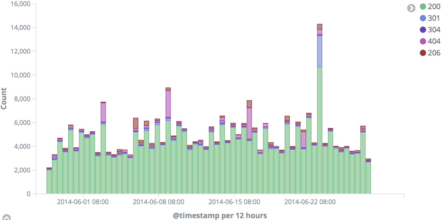
- Analyzing the response codes over time
- Click on
Newand selectVertical Bar - Select
Logstash-*underFrom a New Search, Select Index - In the X axis, select
Date Histogramand@timestampas the field - Click
Add sub-bucketsand selectSplit Series - Select
Termsas the sub aggregation - Select
response.keywordas the field
- Click on
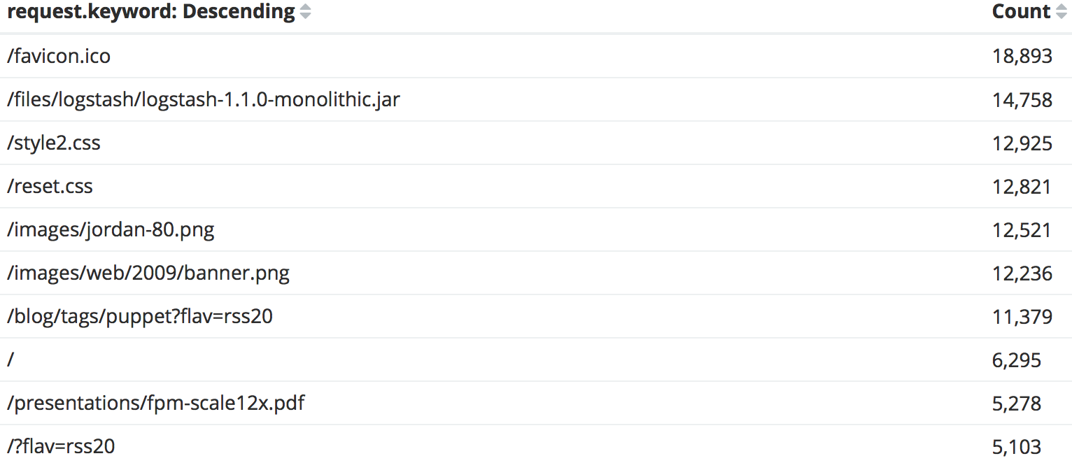
Finding the top 10 URLs requested
新建,选择Data Table,index选择同上。buckets type选择
Split Rows,Aggregation选择Terms,field选择request.keyword,size选择10,结果如下:
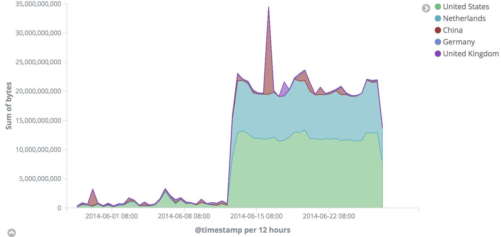
Analyzing the bandwidth usage of the top five countries over time
新建,选择Area,index选择同上。Y轴选择
sum,bytes;X轴选择DateHistogram,@timestamp;sub-buckets选择Split Series,Terms,geoip.country_name.keyword。最后要把sub-buckets拉到X轴前面。这样才是先找到前5的国家,然后对时间轴进行划分。
Finding the most used user agent
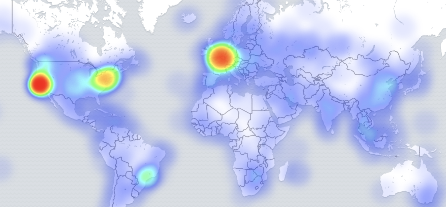
新建,选择Coordinate Map,index选择同上。bucket选择
Geo Coordinates,Geohash,geoip.location, Options处选择Map类型为Heatmap
Analyzing the web traffic originating from different countries
新建,选择Tag Cloud,index选择同上。bucket选择
Tags,Terms,useragent.name.keyword

Dashboards(略)
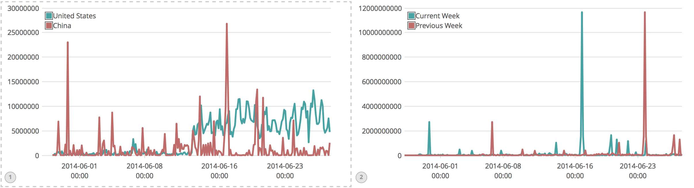
Timelion
中美比较

.es(q='geoip.country_code3:US',metric='avg:bytes').label('United States'), .es(q='geoip.country_code3:CN',metric='avg:bytes').label('China')

与之后一周的比较

.es(q='geoip.country_code3:CN',metric='sum:bytes').label('Current Week'),

.es(q='geoip.country_code3:CN',metric='sum:bytes',

offset=-1w).label('Previous Week')
Metricbeat
metricbeat由modules和metricsets组成。modules定义收集指标的基本逻辑,如连接方式、收集频率、收集哪些指标。每个modules有一到多个metricsets。metricsets是通过给监控对象发送单个请求来收集其列指标的组件,它构建event数据并把数据转移到output。metricbeat的result guarantees是at least once。
好处:
- 即便所监控的对象不能访问,也会返回错误事件
- 整合多个相关指标到单一事件数据
- 会发送元数据,这有利于数据的mapping、确认、查询、过滤等。
- 没有数据转换功能,返回的都是raw data
event structure
{ // 下面@timestamp,metricset,beat的信息是每条常规event都有的。

	"@timestamp": "2017-11-25T11:48:33.269Z",

	"@metadata": {

		"beat": "metricbeat",

		"type": "doc",

		"version": "6.0.0"

	},

	"system": {

		// metric 信息

	},

	"metricset": {

		"name": "xxx", // Name of the metricset that the data is from

		"rtt": 2000, // Round trip time of the request in microseconds

		"module": "system"

	},

	"beat": {

		"version": "6.0.0",

		"name": "SHMN-IN",

		"hostname": "SHMN-IN"

	}

}
配置metricbeat
Module configuration
6.0开始有modules.d目录,里面各个服务都有各自的yml,如mysql.yml,相关配置在里面设置。样式参考system.yml。
General settings :name、tags、max_procs
Output configuration
output.elasticsearch:

 enabled: true

 hosts: ["localhost:9200"]

 username: "elasticuser" # 如果设置了权限

 password: "password"

 pipeline: "ngnix_log_pipeline" # 如果要用ingest node的话

 index: "metricbeat-%{[beat.version]}-%{+yyyy.MM.dd}" # 默认index格式

 # 下面是index的另一种实现。当index被重写时注意要设置setup.dashboards.enabled: false和setup.template.enabled: false,除非提供 setup.template.name 和 setup.template.pattern

 index: "logs-%{+yyyy.MM.dd}"

 indices:

   - index: "debug-%{+yyyy.MM.dd}"

     when.contains:

       message: "DEBUG"

   - index: "error-%{+yyyy.MM.dd}"

     when.contains:

       message: "ERR"

output.logstash:

 hosts: ["localhost:5045", "localhost:5046"]

 loadbalance: true

# 测试

output.console:

 enabled: true

 pretty: true
在metricbeat.yml中开启dashboard功能。这样打开kibana的dashboard就会有默认提供的dashboard模版了。
运行
./metricbeat -e
在Kibana中查看
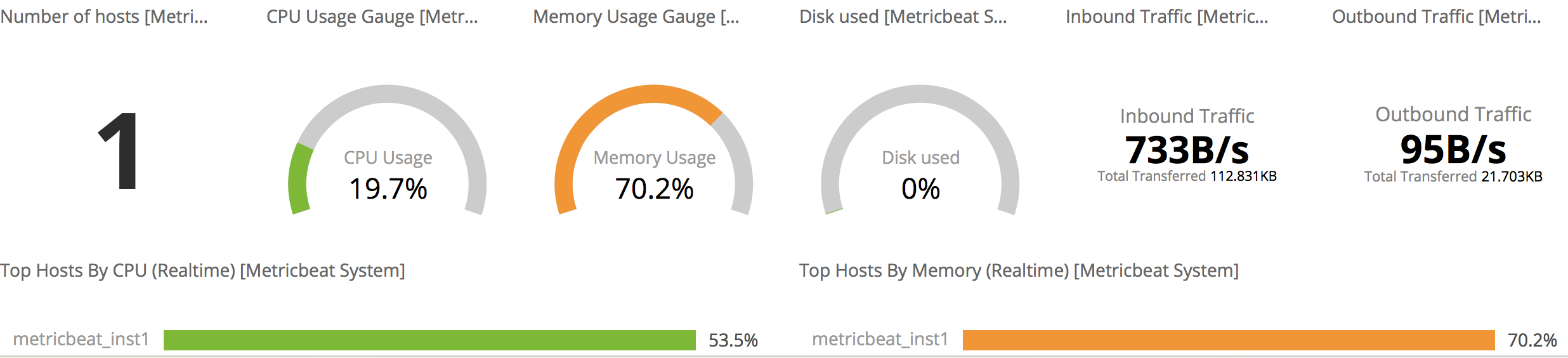
下图为6.0以上的dashboard,需要elasticsearch和kibana都是6.0以上才可以。比5.0的好看不少。
下面是system overview
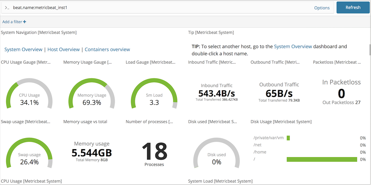
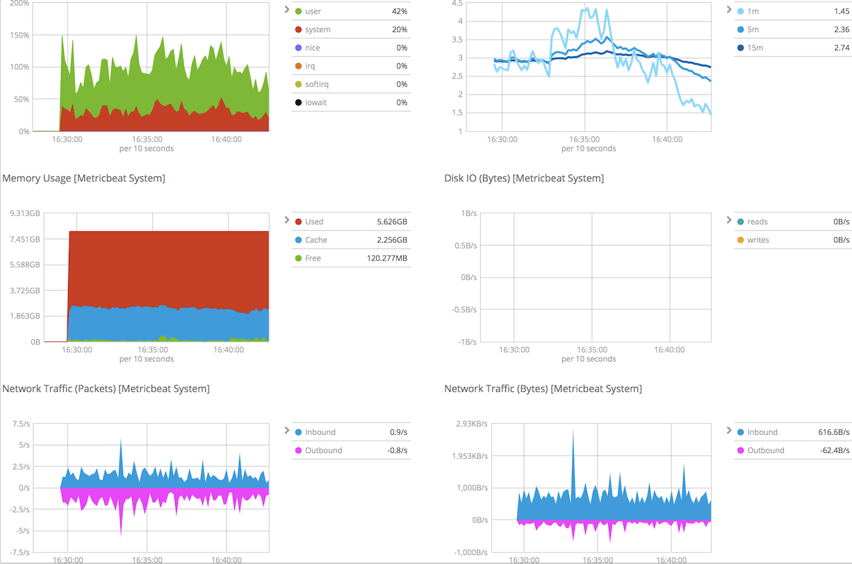
下面是host overview部分信息,注意如果metricbeat.yml的general setting中的那么改变了,要在搜索上写上自己设置的名字。
部署和配置
备份与恢复
在所有节点的elasticsearch.yml文件配置hdfs存储备份的位置path.repo: ["/mount/es_backups"]
然后在此注册文件夹下注册命名存储库,名字下面用backups。

curl -XPUT 'http://localhost:9200/_snapshot/backups' -H 'Content-Type:

application/json' -d '{

 "type": "fs",

 "settings": {

 "location": "/mount/es_backups/backups",

 "compress": true

 }

}'

快照(参考,到时候写进脚本),默认是incremental的。

curl -XPUT

'http://localhost:9200/_snapshot/backups/backup_201710101930?pretty' -H

'Content-Type: application/json' -d'

{

 "indices": "bigginsight,logstash-*",

 "ignore_unavailable": true,

 "include_global_state": false

}'

查看快照

curl -XGET 'http://localhost:9200/_snapshot/backups/_all?pretty'

恢复

curl -XPOST 'http://localhost:9200/_snapshot/backups/backup_201710101930/_restore'
index aliases
生产环境通常是为production index创建链接,并让应用使用这些链接而不是直接使用production index
POST /_aliases

{

 "actions" : [

 { "remove" : { "index" : "index1", "alias" : "current_index" } },

 { "add" : { "index" : "index2", "alias" : "current_index" } }

 ]

}
index templates
设置下面index模版后,每当插入的数据采用新的index,且匹配reading,就会自动执行模版创建index。
PUT _template/readings_template

{

	"index_patterns": ["readings*"], // 任何新索引如果匹配到这个模式就会使用这个模版

	"settings": {

		"number_of_shards": 1

	},

	"mappings": {

		"reading": {

			"properties": {

				"sensorId": {

					"type": "keyword"

				},

				"timestamp": {

					"type": "date"

				},

				"reading": {

					"type": "double"

				}

			}

		}

	}

}
时间序列数据
一个index存储大量时间序列数据并非好事,通常以时间,如天、周作为单位新增索引。这主要考虑到shard数量、mapping的变化、过时数据的处理:
shard数量
需要根据当前业务的数据量来估计,但shard一旦设定就不能修改了。不合理的shard数量会影响相关评分和聚合准确度:
- 评分:相对频率是基于各个分片内而不是基于所有分片。
- 聚合:聚合同样是基于各个分片,例如top10则取个分片的top10。如果某个bucket位于其中一个分片返回的前n个bucket中,并且该bucket不是任何其他分片的前n个bucket之一,则协调节点聚合的最终计数会忽略这个bucket。
mapping的变化
随着业务的变化,fields可能会增加,有些fields会过时,过多deprecated field耗费资源
其他
client.transport.sniff为true来使客户端去嗅探整个集群的状态,把集群中其它机器的ip地址自动加到客户端中
当ES服务器监听使用内网服务器IP而访问使用外网IP时,不要使用client.transport.sniff为true,在自动发现时会使用内网IP进行通信,导致无法连接到ES服务器,而直接使用addTransportAddress方法进行指定ES服务器。
// 一些优化说明

post

localhost:9200/index_name/type_name/_search?explain=true

禁止删除索引时使用通配符

put + http://<ip>:<port>/_cluster/settings 动态方式改设置

{

    "transient": {

        "action.destructive_requires_name": true

    }

}

put + http://<ip>:<port>/_all/_settings?preserve_existing=true

{

    index.refresh_interval: "30s"

}

非动态改设置,即在config文件中改

discovery.zen.fd.ping_interval: 10s

discovery.zen.fd.ping_timemout: 120s

discovery.zen.fd.ping_retries: 3

master节点一般不存储数据

node.master: true

node.data: false

针对数据节点,关闭http功能。从而减少一些插件安装到这些节点,浪费资源。

http.enable: false

负载均衡节点:master和data都为false,但一般不用自带的

内存设定:JVM针对内存小于32G才会优化,所以每个节点不要大于这个值。另外堆内存至少小于可用内存的50%,留空间给Apache Lucene。

写入数据从index改为bulk
参考:
Learning Elastic Stack 6.0
最新文章
- XML基础
- HTML5模仿逼真地球自转
- C++笔记(一)
- MXNet 学习 (1) --- 最易上手的深度学习开源库 --- 安装及环境搭建
- HTTPS的七个误解
- BZOJ 2292 永远挑战
- ViewPager的监听事件失效
- 【M5】对定制的“类型转换函数”保持警觉
- tomcat6.0添加ssi(*.shtml)配置
- FL2440移植Linux2.6.33.7内核
- css3购物网站商品文字提示实例
- License制作
- angularJS 系列(七)---指令
- Android启动脚本init.rc(2)
- Android新手入门
- docker - win7下构建swarm nodes实现跨host的容器之间的通信
- 【Android 应用开发】Android - 按钮组件详解
- 从壹开始前后端分离 [.netCore 填坑 ] 三十四║Swagger:API多版本控制,带来的思考
- Python——Django-urls.py的作用
- Linux 学习笔记 3:Shell 基础