Regularization

Deep Learning models have so much flexibility and capacity that overfitting can be a serious problem，if the training dataset is not big enough. Sure it does well on the training set, but the learned network doesn't generalize to new examples that it has never seen!（它在训练集上工作很好，但是不能用于它从未见过的新样例）

You will learn to: Use regularization in your deep learning models.

Let's first import the packages you are going to use.

# import packages

import numpy as np

import matplotlib.pyplot as plt

from reg_utils import sigmoid, relu, plot_decision_boundary, initialize_parameters, load_2D_dataset, predict_dec

from reg_utils import compute_cost, predict, forward_propagation, backward_propagation, update_parameters

import sklearn

import sklearn.datasets

import scipy.io

from testCases import *

%matplotlib inline

plt.rcParams['figure.figsize'] = (7.0, 4.0) # set default size of plots

plt.rcParams['image.interpolation'] = 'nearest'

plt.rcParams['image.cmap'] = 'gray'

Problem Statement: You have just been hired as an AI expert by the French Football Corporation. They would like you to recommend positions where France's goal keeper should kick the ball so that the French team's players can then hit it with their head.

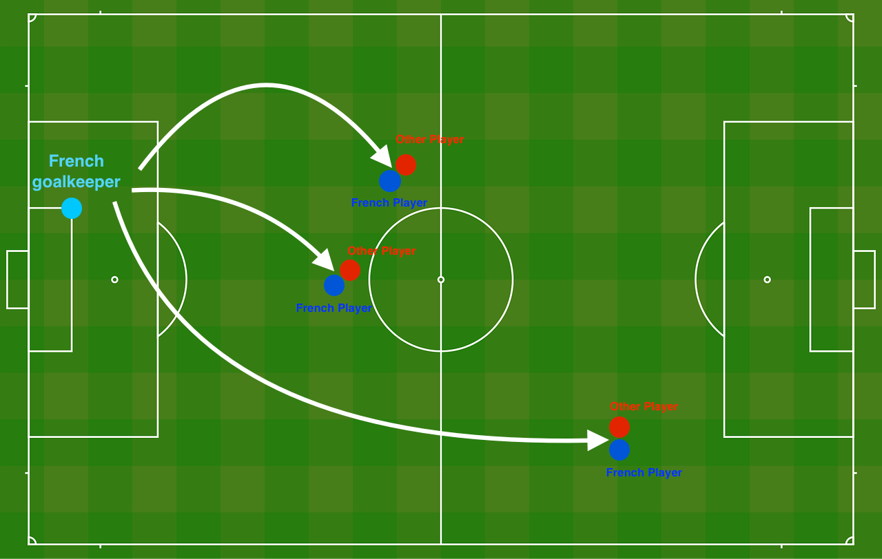
**Figure 1** : **Football field**
The goal keeper kicks the ball in the air, the players of each team are fighting to hit the ball with their head

They give you the following 2D dataset from France's past 10 games.

train_X, train_Y, test_X, test_Y = load_2D_dataset()

Each dot corresponds to a position on the football field where a football player has hit the ball with his/her head after the French goal keeper has shot the ball from the left side of the football field.

If the dot is blue, it means the French player managed to hit the ball with his/her head(蓝色：法国接到球)
If the dot is red, it means the other team's player hit the ball with their head (红色：法国接不到)

Your goal: Use a deep learning model to find the positions on the field where the goalkeeper should kick the ball.

Analysis of the dataset: This dataset is a little noisy, but it looks like a diagonal line separating the upper left half (blue) from the lower right half (red) would work well.

You will first try a non-regularized model. Then you'll learn how to regularize it and decide which model you will choose to solve the French Football Corporation's problem.

1 - Non-regularized model

You will use the following neural network (already implemented for you below). This model can be used:

in regularization mode -- by setting the lambd input to a non-zero value. We use "lambd" instead of "lambda" because "lambda" is a reserved keyword in Python.
in dropout mode -- by setting the keep_prob to a value less than one

You will first try the model without any regularization. Then, you will implement:

L2 regularization -- functions: "compute_cost_with_regularization()" and "backward_propagation_with_regularization()"
Dropout -- functions: "forward_propagation_with_dropout()" and "backward_propagation_with_dropout()"

In each part, you will run this model with the correct inputs so that it calls the functions you've implemented. Take a look at the code below to familiarize yourself with the model.

def model(X, Y, learning_rate = 0.3, num_iterations = 30000, print_cost = True, lambd = 0, keep_prob = 1):

    """

    Implements a three-layer neural network: LINEAR->RELU->LINEAR->RELU->LINEAR->SIGMOID.

    Arguments:

    X -- input data, of shape (input size, number of examples)

    Y -- true "label" vector (1 for blue dot / 0 for red dot), of shape (output size, number of examples)

    learning_rate -- learning rate of the optimization

    num_iterations -- number of iterations of the optimization loop

    print_cost -- If True, print the cost every 10000 iterations

    lambd -- regularization hyperparameter, scalar

    keep_prob - probability of keeping a neuron active during drop-out, scalar.

    Returns:

    parameters -- parameters learned by the model. They can then be used to predict.

    """

    grads = {}

    costs = []                            # to keep track of the cost

    m = X.shape[1]                        # number of examples

    layers_dims = [X.shape[0], 20, 3, 1]

    # Initialize parameters dictionary.

    parameters = initialize_parameters(layers_dims)

    # Loop (gradient descent)

    for i in range(0, num_iterations):

        # Forward propagation: LINEAR -> RELU -> LINEAR -> RELU -> LINEAR -> SIGMOID.

        if keep_prob == 1:

            a3, cache = forward_propagation(X, parameters)

        elif keep_prob < 1:         # dropout正则化

            a3, cache = forward_propagation_with_dropout(X, parameters, keep_prob)

        # Cost function

        if lambd == 0:

            cost = compute_cost(a3, Y)

        else:                      # 使用 L2正则化时，计算的cost

            cost = compute_cost_with_regularization(a3, Y, parameters, lambd)

        # Backward propagation.

        assert(lambd==0 or keep_prob==1)      # it is possible to use both L2 regularization and dropout,

                                               # but this assignment will only explore one at a time

        if lambd == 0 and keep_prob == 1:     # 什么正则化都没有用，普通的反向传播

            grads = backward_propagation(X, Y, cache)

        elif lambd != 0:                      # L2 正则化

            grads = backward_propagation_with_regularization(X, Y, cache, lambd)

        elif keep_prob < 1:                   # dropout正则化

            grads = backward_propagation_with_dropout(X, Y, cache, keep_prob)

        # Update parameters.

        parameters = update_parameters(parameters, grads, learning_rate)

        # Print the loss every 10000 iterations

        if print_cost and i % 10000 == 0:

            print("Cost after iteration {}: {}".format(i, cost))

        if print_cost and i % 1000 == 0:

            costs.append(cost)

    # plot the cost

    plt.plot(costs)

    plt.ylabel('cost')

    plt.xlabel('iterations (x1,000)')

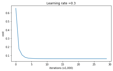
    plt.title("Learning rate =" + str(learning_rate))

    plt.show()

    return parameters

Let's train the model without any regularization, and observe the accuracy on the train/test sets.

parameters = model(train_X, train_Y)

print ("On the training set:")

predictions_train = predict(train_X, train_Y, parameters)

print ("On the test set:")

predictions_test = predict(test_X, test_Y, parameters)

Cost after iteration 0: 0.6557412523481002

Cost after iteration 10000: 0.1632998752572419

Cost after iteration 20000: 0.13851642423239133

On the training set:

Accuracy: 0.9478672985781991

On the test set:

Accuracy: 0.915

The train accuracy is 94.8% while the test accuracy is 91.5%. This is the baseline model (you will observe the impact of regularization on this model). Run the following code to plot the decision boundary of your model.

plt.title("Model without regularization")

axes = plt.gca()

axes.set_xlim([-0.75,0.40])

axes.set_ylim([-0.75,0.65])

plot_decision_boundary(lambda x: predict_dec(parameters, x.T), train_X, train_Y)

非正则化模型，明显的过拟合了！下面介绍两个技术来减少过拟合.

2 - L2 Regularization

The standard way to avoid overfitting is called L2 regularization. It consists of appropriately modifying your cost function, from:

\[J = -\frac{1}{m} \sum\limits_{i = 1}^{m} \large{(}\small y^{(i)}\log\left(a^{[L](i)}\right) + (1-y^{(i)})\log\left(1- a^{[L](i)}\right) \large{)} \tag{1}
\]

To:

\[J_{regularized} = \small \underbrace{-\frac{1}{m} \sum\limits_{i = 1}^{m} \large{(}\small y^{(i)}\log\left(a^{[L](i)}\right) + (1-y^{(i)})\log\left(1- a^{[L](i)}\right) \large{)} }_\text{cross-entropy cost} + \underbrace{\frac{1}{m} \frac{\lambda}{2} \sum\limits_l\sum\limits_k\sum\limits_j W_{k,j}^{[l]2} }_\text{L2 regularization cost} \tag{2}
\]

Let's modify your cost and observe the consequences.

Exercise: Implement compute_cost_with_regularization() which computes the cost given by formula (2). To calculate $\sum\limits_k\sum\limits_j W_{k,j}^{[l]2}$ , use :

np.sum(np.square(Wl))

Note that you have to do this for $W^{[1]}$, $W^{[2]}$ and $W^{[3]}$, then sum the three terms and multiply by $ \frac{1}{m} \frac{\lambda}{2} $.

# GRADED FUNCTION: compute_cost_with_regularization

def compute_cost_with_regularization(A3, Y, parameters, lambd):

    """

    Implement the cost function with L2 regularization. See formula (2) above.

    Arguments:

    A3 -- post-activation, output of forward propagation, of shape (output size, number of examples)

    Y -- "true" labels vector, of shape (output size, number of examples)

    parameters -- python dictionary containing parameters of the model

    Returns:

    cost - value of the regularized loss function (formula (2))

    """

    m = Y.shape[1]

    W1 = parameters["W1"]

    W2 = parameters["W2"]

    W3 = parameters["W3"]

    cross_entropy_cost = compute_cost(A3, Y) # This gives you the cross-entropy part of the cost

    ### START CODE HERE ### (approx. 1 line)

    L2_regularization_cost = (1. / m)*(lambd / 2) * (np.sum(np.square(W1)) + np.sum(np.square(W2)) + np.sum(np.square(W3)))

    ### END CODER HERE ###

    cost = cross_entropy_cost + L2_regularization_cost

    return cost

A3, Y_assess, parameters = compute_cost_with_regularization_test_case()

print("cost = " + str(compute_cost_with_regularization(A3, Y_assess, parameters, lambd = 0.1)))

输出：

cost = 1.7864859451590758、

Of course, because you changed the cost, you have to change backward propagation as well! All the gradients have to be computed with respect to this new cost.

Exercise: Implement the changes needed in backward propagation to take into account regularization. The changes only concern dW1, dW2 and dW3. For each, you have to add the regularization term's gradient ($\frac{d}{dW} ( \frac{1}{2}\frac{\lambda}{m} W^2) = \frac{\lambda}{m} W$).

注：就是在以往的梯度后面，再加一个$\frac{\lambda}{m} W$）

# GRADED FUNCTION: backward_propagation_with_regularization

def backward_propagation_with_regularization(X, Y, cache, lambd):

    """

    Implements the backward propagation of our baseline model to which we added an L2 regularization.

    Arguments:

    X -- input dataset, of shape (input size, number of examples)

    Y -- "true" labels vector, of shape (output size, number of examples)

    cache -- cache output from forward_propagation()

    lambd -- regularization hyperparameter, scalar

    Returns:

    gradients -- A dictionary with the gradients with respect to each parameter, activation and pre-activation variables

    """

    m = X.shape[1]

    (Z1, A1, W1, b1, Z2, A2, W2, b2, Z3, A3, W3, b3) = cache

    dZ3 = A3 - Y

    ### START CODE HERE ### (approx. 1 line)

    dW3 = 1./m * (np.dot(dZ3, A2.T) + lambd * W3)

    ### END CODE HERE ###

    db3 = 1./m * np.sum(dZ3, axis=1, keepdims = True)

    dA2 = np.dot(W3.T, dZ3)

    dZ2 = np.multiply(dA2, np.int64(A2 > 0))

    ### START CODE HERE ### (approx. 1 line)

    dW2 = 1./m * (np.dot(dZ2, A1.T) + lambd * W2 )

    ### END CODE HERE ###

    db2 = 1./m * np.sum(dZ2, axis=1, keepdims = True)

    dA1 = np.dot(W2.T, dZ2)

    dZ1 = np.multiply(dA1, np.int64(A1 > 0))

    ### START CODE HERE ### (approx. 1 line)

    dW1 = 1./m * (np.dot(dZ1, X.T) + lambd * W1 )

    ### END CODE HERE ###

    db1 = 1./m * np.sum(dZ1, axis=1, keepdims = True)

    gradients = {"dZ3": dZ3, "dW3": dW3, "db3": db3,"dA2": dA2,

                 "dZ2": dZ2, "dW2": dW2, "db2": db2, "dA1": dA1,

                 "dZ1": dZ1, "dW1": dW1, "db1": db1}

    return gradients

X_assess, Y_assess, cache = backward_propagation_with_regularization_test_case()

grads = backward_propagation_with_regularization(X_assess, Y_assess, cache, lambd = 0.7)

print ("dW1 = "+ str(grads["dW1"]))

print ("dW2 = "+ str(grads["dW2"]))

print ("dW3 = "+ str(grads["dW3"]))

dW1 = [[-0.25604646 0.12298827 -0.28297129]

[-0.17706303 0.34536094 -0.4410571 ]]

dW2 = [[ 0.79276486 0.85133918]

[-0.0957219 -0.01720463]

[-0.13100772 -0.03750433]]

dW3 = [[-1.77691347 -0.11832879 -0.09397446]]

Let's now run the model with L2 regularization $(\lambda = 0.7)$. The model() function will call:

compute_cost_with_regularization instead of compute_cost
backward_propagation_with_regularization instead of backward_propagation

Cost after iteration 0: 0.6974484493131264

Cost after iteration 10000: 0.2684918873282239

Cost after iteration 20000: 0.26809163371273004

On the train set:

Accuracy: 0.9383886255924171

On the test set:

Accuracy: 0.93

现在，已经不过拟合了，下面绘制决策边界

plt.title("Model with L2-regularization")

axes = plt.gca()

axes.set_xlim([-0.75,0.40])

axes.set_ylim([-0.75,0.65])

plot_decision_boundary(lambda x: predict_dec(parameters, x.T), train_X, train_Y)

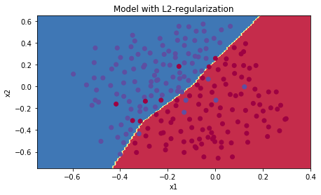
Observations:

$\lambda$：是你可以在验证集（dev set）上调整的超参数（hyperparameter）
L2正则化让你的决策边界十分的平滑。如果 $\lambda$很大，很可能过于光滑，导致高偏差模型（即：训练集和测试集误差都高，欠拟合）

L2-regularization 真正做了什么？:

L2-regularization 依赖于假设，小权重的模型比大权重的模型简单. 因此，通过惩罚代价函数的平方值的权重，使所有权重变成更小的值（更新参数的时候）【权重衰减（weight decay）】。有大的权重将会变得更大的代价。它会导致一个更平滑的模型，其中输出随着随着输入的变化，而变得更加缓慢。

What you should remember -- the implications of L2-regularization on:

The cost computation:
- A regularization term is added to the cost
The backpropagation function:
- There are extra terms in the gradients with respect to weight matrices
Weights end up smaller ("weight decay"):
- Weights are pushed to smaller values.

3 - Dropout

Finally, dropout is a widely used regularization technique that is specific to deep learning.

It randomly shuts down some neurons in each iteration. Watch these two videos to see what this means!

Figure 2 : Drop-out on the second hidden layer.

At each iteration, you shut down (= set to zero) each neuron of a layer with probability $1 - keep\_prob$ or keep it with probability $keep\_prob$ (50% here). The dropped neurons don't contribute to the training in both the forward and backward propagations of the iteration.

Figure 3 : Drop-out on the first and third hidden layers.

$1^{st}$ layer: we shut down on average 40% of the neurons. $3^{rd}$ layer: we shut down on average 20% of the neurons.

当你shut down一些神经元，你实际修改了你的模型。

在每次迭代后，你训练一个不同的模型，只使用你神经元里的子集

在dropout后，你的神经元因此变得对特定的神经元的激励，不那么敏感，因为这些神经元随时可能会被shut down。

3.1 - Forward propagation with dropout

Exercise: Implement the forward propagation with dropout. You are using a 3 layer neural network, and will add dropout to the first and second hidden layers. We will not apply dropout to the input layer or output layer.

Instructions:

You would like to shut down some neurons in the first and second layers. To do that, you are going to carry out 4 Steps:

initialize matrix D1 = np.random.rand(..., ...)
convert entries of D1 to 0 or 1 (using keep_prob as the threshold)
shut down some neurons of A1 (np.multiply(A1, D1)
$A^{[1]}$ /= keep_prob. 因为有1−keep_prob1 的单元失活了，这样$a3$的期望值也就减少了1−keep_prob1，所以我们要用a3/keep_proba3，这样a3的期望值不变。这就是inverted dropout。参考

# GRADED FUNCTION: forward_propagation_with_dropout

def forward_propagation_with_dropout(X, parameters, keep_prob = 0.5):

    """

    Implements the forward propagation: LINEAR -> RELU + DROPOUT -> LINEAR -> RELU + DROPOUT -> LINEAR -> SIGMOID.

    Arguments:

    X -- input dataset, of shape (2, number of examples)

    parameters -- python dictionary containing your parameters "W1", "b1", "W2", "b2", "W3", "b3":

                    W1 -- weight matrix of shape (20, 2)

                    b1 -- bias vector of shape (20, 1)

                    W2 -- weight matrix of shape (3, 20)

                    b2 -- bias vector of shape (3, 1)

                    W3 -- weight matrix of shape (1, 3)

                    b3 -- bias vector of shape (1, 1)

    keep_prob - probability of keeping a neuron active during drop-out, scalar

    Returns:

    A3 -- last activation value, output of the forward propagation, of shape (1,1)

    cache -- tuple, information stored for computing the backward propagation

    """

    np.random.seed(1)

    # retrieve parameters

    W1 = parameters["W1"]

    b1 = parameters["b1"]

    W2 = parameters["W2"]

    b2 = parameters["b2"]

    W3 = parameters["W3"]

    b3 = parameters["b3"]

    # LINEAR -> RELU -> LINEAR -> RELU -> LINEAR -> SIGMOID

    Z1 = np.dot(W1, X) + b1

    A1 = relu(Z1)

    ### START CODE HERE ### (approx. 4 lines)         # Steps 1-4 below correspond to the Steps 1-4 described above.

    D1 = np.random.rand(A1.shape[0], A1.shape[1])     # Step 1: initialize matrix D1 = np.random.rand(..., ...)

    D1 = D1 < keep_prob                               # Step 2: convert entries of D1 to 0 or 1 (using keep_prob as the threshold)

    A1 = np.multiply(A1, D1)                          # Step 3: shut down some neurons of A1

    A1 /= keep_prob                                   # Step 4: scale the value of neurons that haven't been shut down

    ### END CODE HERE ###

    Z2 = np.dot(W2, A1) + b2

    A2 = relu(Z2)

    ### START CODE HERE ### (approx. 4 lines)

    D2 = np.random.rand(A2.shape[0], A2.shape[1])               # Step 1: initialize matrix D2 = np.random.rand(..., ...)

    D2 = D2 < keep_prob                                         # Step 2: convert entries of D2 to 0 or 1 (using keep_prob as the threshold)

    A2 = np.multiply(A2, D2)                                    # Step 3: shut down some neurons of A2

    A2 /= keep_prob                                             # Step 4: scale the value of neurons that haven't been shut down

    ### END CODE HERE ###

    Z3 = np.dot(W3, A2) + b3

    A3 = sigmoid(Z3)

    cache = (Z1, D1, A1, W1, b1, Z2, D2, A2, W2, b2, Z3, A3, W3, b3)

    return A3, cache

X_assess, parameters = forward_propagation_with_dropout_test_case()

A3, cache = forward_propagation_with_dropout(X_assess, parameters, keep_prob = 0.7)

print ("A3 = " + str(A3))

A3 = [[0.36974721 0.00305176 0.04565099 0.49683389 0.36974721]]

3.2 - Backward propagation with dropout

Exercise: Implement the backward propagation with dropout. As before, you are training a 3 layer network. Add dropout to the first and second hidden layers, using the masks $D^{[1]}$ and $D^{[2]}$ stored in the cache.

Instruction:

Backpropagation with dropout is actually quite easy. You will have to carry out 2 Steps:

Apply mask D2 to shut down the same neurons as during the forward propagation (By reapplying the same mask $D^{[1]}$ to dA1)
Scale the value of neurons that haven't been shut down. ($dA^{[1]}$ /= keep_prob)

# GRADED FUNCTION: backward_propagation_with_dropout

def backward_propagation_with_dropout(X, Y, cache, keep_prob):

    """

    Implements the backward propagation of our baseline model to which we added dropout.

    Arguments:

    X -- input dataset, of shape (2, number of examples)

    Y -- "true" labels vector, of shape (output size, number of examples)

    cache -- cache output from forward_propagation_with_dropout()

    keep_prob - probability of keeping a neuron active during drop-out, scalar

    Returns:

    gradients -- A dictionary with the gradients with respect to each parameter, activation and pre-activation variables

    """

    m = X.shape[1]

    (Z1, D1, A1, W1, b1, Z2, D2, A2, W2, b2, Z3, A3, W3, b3) = cache

    dZ3 = A3 - Y

    dW3 = 1./m * np.dot(dZ3, A2.T)

    db3 = 1./m * np.sum(dZ3, axis=1, keepdims = True)

    dA2 = np.dot(W3.T, dZ3)

    ### START CODE HERE ### (≈ 2 lines of code)

    dA2 = np.multiply(dA2, D2)              # Step 1: Apply mask D2 to shut down the same neurons as during the forward propagation

    dA2 /= keep_prob                       # Step 2: Scale the value of neurons that haven't been shut down

    ### END CODE HERE ###

    dZ2 = np.multiply(dA2, np.int64(A2 > 0))

    dW2 = 1./m * np.dot(dZ2, A1.T)

    db2 = 1./m * np.sum(dZ2, axis=1, keepdims = True)

    dA1 = np.dot(W2.T, dZ2)

    ### START CODE HERE ### (≈ 2 lines of code)

    dA1 = np.multiply(dA1, D1)             # Step 1: Apply mask D1 to shut down the same neurons as during the forward propagation

    dA1 /= keep_prob            # Step 2: Scale the value of neurons that haven't been shut down

    ### END CODE HERE ###

    dZ1 = np.multiply(dA1, np.int64(A1 > 0))

    dW1 = 1./m * np.dot(dZ1, X.T)

    db1 = 1./m * np.sum(dZ1, axis=1, keepdims = True)

    gradients = {"dZ3": dZ3, "dW3": dW3, "db3": db3,"dA2": dA2,

                 "dZ2": dZ2, "dW2": dW2, "db2": db2, "dA1": dA1,

                 "dZ1": dZ1, "dW1": dW1, "db1": db1}

    return gradients

X_assess, Y_assess, cache = backward_propagation_with_dropout_test_case()

gradients = backward_propagation_with_dropout(X_assess, Y_assess, cache, keep_prob = 0.8)

print ("dA1 = " + str(gradients["dA1"]))

print ("dA2 = " + str(gradients["dA2"]))

dA1 = [[ 0.36544439 0. -0.00188233 0. -0.17408748]

[ 0.65515713 0. -0.00337459 0. -0. ]]

dA2 = [[ 0.58180856 0. -0.00299679 0. -0.27715731]

[ 0. 0.53159854 -0. 0.53159854 -0.34089673]

[ 0. 0. -0.00292733 0. -0. ]]

Let's now run the model with dropout (keep_prob = 0.86). It means at every iteration you shut down each neurons of layer 1 and 2 with 14% probability. The function model() will now call: （应用到模型）

forward_propagation_with_dropout instead of forward_propagation.
backward_propagation_with_dropout instead of backward_propagation.

parameters = model(train_X, train_Y, keep_prob = 0.86, learning_rate = 0.3)

print ("On the train set:")

predictions_train = predict(train_X, train_Y, parameters)

print ("On the test set:")

predictions_test = predict(test_X, test_Y, parameters)

Cost after iteration 0: 0.6543912405149825

Cost after iteration 10000: 0.061016986574905605

Cost after iteration 20000: 0.060582435798513114

On the train set:

Accuracy: 0.9289099526066351

On the test set:

Accuracy: 0.95

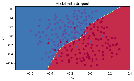
成功的解决了过拟合！

绘制决策边界

plt.title("Model with dropout")

axes = plt.gca()

axes.set_xlim([-0.75,0.40])

axes.set_ylim([-0.75,0.65])

plot_decision_boundary(lambda x: predict_dec(parameters, x.T), train_X, train_Y)

Note:

A common mistake when using dropout is to use it both in training and testing. 你应该只在训练集使用dropout！
Deep learning frameworks like tensorflow, PaddlePaddle, keras or caffe come with a dropout layer implementation. Don't stress - you will soon learn some of these frameworks.

What you should remember about dropout:

Dropout is a regularization technique.
You only use dropout during training. Don't use dropout (randomly eliminate nodes) during test time.
Apply dropout both during forward and backward propagation.
在训练集时，每一个 dropout layer / keep_prob 来保持激励(activation)输出同样的期望值. For example, if keep_prob is 0.5, then we will on average shut down half the nodes, 因此输出被减少了一半，因此只剩下一半来贡献解决方案. A / 0.5 == A * 2. 因此，输出现在有同样的期望值.

4 - conclusions

Here are the results of our three models:

model	train accuracy	test accuracy
3-layer NN without regularization	95%	91.5%
3-layer NN with L2-regularization	94%	93%
3-layer NN with dropout	93%	95%

注意：正则化伤害了训练集的性能，这是因为它限制了网络网络，过度拟合的能力。但他提供了更好的测试集精度。

巴特西

改善深层神经网络-week1编程题（Regularization）