Elasticsearch基本概念和使用
Elasticsearch基本概念和使用
1.操作索引
1.1.基本概念
Elasticsearch也是基于Lucene的全文检索库,本质也是存储数据,很多概念与MySQL类似的。
对比关系:
索引(indices)--------------------------------Databases 数据库
类型(type)-----------------------------Table 数据表
文档(Document)----------------Row 行
字段(Field)-------------------Columns 列
详细说明:
| 概念 | 说明 |
|---|---|
| 索引库(indices) | indices是index的复数,代表许多的索引, |
| 类型(type) | 类型是模拟mysql中的table概念,一个索引库下可以有不同类型的索引,比如商品索引,订单索引,其数据格式不同。不过这会导致索引库混乱,因此未来版本中会移除这个概念 |
| 文档(document) | 存入索引库原始的数据。比如每一条商品信息,就是一个文档 |
| 字段(field) | 文档中的属性 |
| 映射配置(mappings) | 字段的数据类型、属性、是否索引、是否存储等特性 |
是不是与Lucene和solr中的概念类似。
另外,在SolrCloud中,有一些集群相关的概念,在Elasticsearch也有类似的:
- 索引集(Indices,index的复数):逻辑上的完整索引
- 分片(shard):数据拆分后的各个部分
- 副本(replica):每个分片的复制
要注意的是:Elasticsearch本身就是分布式的,因此即便你只有一个节点,Elasticsearch默认也会对你的数据进行分片和副本操作,当你向集群添加新数据时,数据也会在新加入的节点中进行平衡。
1.2.创建索引
1.2.1.语法
Elasticsearch采用Rest风格API,因此其API就是一次http请求,你可以用任何工具发起http请求
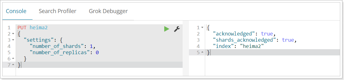
创建索引的请求格式:
请求方式:PUT
请求路径:/索引库名
请求参数:json格式:
{

    "settings": {

        "number_of_shards": 3,

        "number_of_replicas": 2

      }

}
- settings:索引库的设置
- number_of_shards:分片数量
- number_of_replicas:副本数量
- settings:索引库的设置
1.2.2.测试
我们先用RestClient来试试

响应:

可以看到索引创建成功了。
1.2.3.使用kibana创建
kibana的控制台,可以对http请求进行简化,示例:
相当于是省去了elasticsearch的服务器地址
而且还有语法提示,非常舒服。
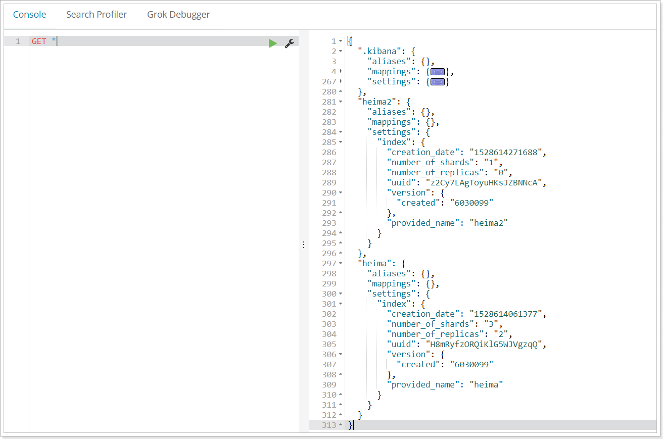
1.3.查看索引设置
语法
Get请求可以帮我们查看索引信息,格式:
GET /索引库名

或者,我们可以使用*来查询所有索引库配置:
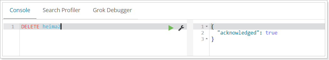
1.4.删除索引
删除索引使用DELETE请求
语法
DELETE /索引库名
示例
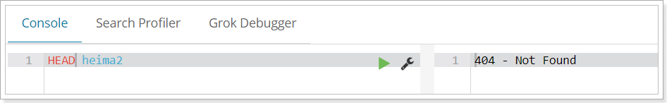
再次查看heima2:

当然,我们也可以用HEAD请求,查看索引是否存在:
1.5.映射配置
索引有了,接下来肯定是添加数据。但是,在添加数据之前必须定义映射。
什么是映射?
映射是定义文档的过程,文档包含哪些字段,这些字段是否保存,是否索引,是否分词等
只有配置清楚,Elasticsearch才会帮我们进行索引库的创建(不一定)
1.5.1.创建映射字段
语法
请求方式依然是PUT
PUT /索引库名/_mapping/类型名称

{

  "properties": {

    "字段名": {

      "type": "类型",

      "index": true,

      "store": true,

      "analyzer": "分词器"

    }

  }

}
- 类型名称:就是前面将的type的概念,类似于数据库中的不同表
字段名:任意填写 ,可以指定许多属性,例如: - type:类型,可以是text、long、short、date、integer、object等
- index:是否索引,默认为true
- store:是否存储,默认为false
- analyzer:分词器,这里的
ik_max_word即使用ik分词器
示例
发起请求:
PUT heima/_mapping/goods

{

  "properties": {

    "title": {

      "type": "text",

      "analyzer": "ik_max_word"

    },

    "images": {

      "type": "keyword",

      "index": "false"

    },

    "price": {

      "type": "float"

    }

  }

}
响应结果:
{

  "acknowledged": true

}
1.5.2.查看映射关系
语法:
GET /索引库名/_mapping
示例:
GET /heima/_mapping
响应:
{

  "heima": {

    "mappings": {

      "goods": {

        "properties": {

          "images": {

            "type": "keyword",

            "index": false

          },

          "price": {

            "type": "float"

          },

          "title": {

            "type": "text",

            "analyzer": "ik_max_word"

          }

        }

      }

    }

  }

}
1.5.3.字段属性详解
1.5.3.1.type
Elasticsearch中支持的数据类型非常丰富:

我们说几个关键的:
String类型,又分两种:
- text:可分词,不可参与聚合
- keyword:不可分词,数据会作为完整字段进行匹配,可以参与聚合
Numerical:数值类型,分两类
- 基本数据类型:long、interger、short、byte、double、float、half_float
- 浮点数的高精度类型:scaled_float
- 需要指定一个精度因子,比如10或100。elasticsearch会把真实值乘以这个因子后存储,取出时再还原。
Date:日期类型
elasticsearch可以对日期格式化为字符串存储,但是建议我们存储为毫秒值,存储为long,节省空间。
1.5.3.2.index
index影响字段的索引情况。
- true:字段会被索引,则可以用来进行搜索。默认值就是true
- false:字段不会被索引,不能用来搜索
index的默认值就是true,也就是说你不进行任何配置,所有字段都会被索引。
但是有些字段是我们不希望被索引的,比如商品的图片信息,就需要手动设置index为false。
1.5.3.3.store
是否将数据进行额外存储。
在学习lucene和solr时,我们知道如果一个字段的store设置为false,那么在文档列表中就不会有这个字段的值,用户的搜索结果中不会显示出来。
但是在Elasticsearch中,即便store设置为false,也可以搜索到结果。
原因是Elasticsearch在创建文档索引时,会将文档中的原始数据备份,保存到一个叫做_source的属性中。而且我们可以通过过滤_source来选择哪些要显示,哪些不显示。
而如果设置store为true,就会在_source以外额外存储一份数据,多余,因此一般我们都会将store设置为false,事实上,store的默认值就是false。
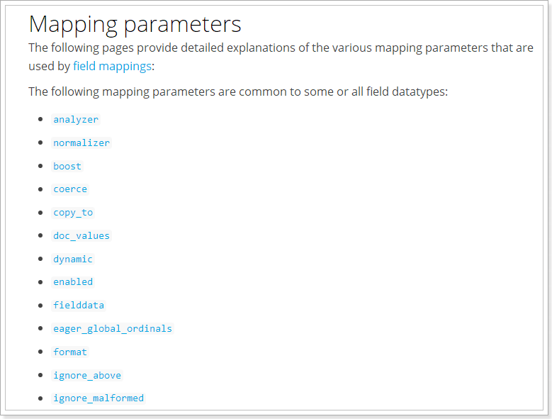
1.5.3.4.boost
激励因子,这个与lucene中一样
其它的不再一一讲解,用的不多,大家参考官方文档:
1.6.新增数据
1.6.1.随机生成id
通过POST请求,可以向一个已经存在的索引库中添加数据。
语法:
POST /索引库名/类型名

{

    "key":"value"

}
示例:
POST /heima/goods/

{

    "title":"小米手机",

    "images":"http://image.leyou.com/12479122.jpg",

    "price":2699.00

}
响应:
{

  "_index": "heima",

  "_type": "goods",

  "_id": "r9c1KGMBIhaxtY5rlRKv",

  "_version": 1,

  "result": "created",

  "_shards": {

    "total": 3,

    "successful": 1,

    "failed": 0

  },

  "_seq_no": 0,

  "_primary_term": 2

}
通过kibana查看数据:
get _search

{

    "query":{

        "match_all":{}

    }

}
{

  "_index": "heima",

  "_type": "goods",

  "_id": "r9c1KGMBIhaxtY5rlRKv",

  "_version": 1,

  "_score": 1,

  "_source": {

    "title": "小米手机",

    "images": "http://image.leyou.com/12479122.jpg",

    "price": 2699

  }

}
_source:源文档信息,所有的数据都在里面。_id:这条文档的唯一标示,与文档自己的id字段没有关联
1.6.2.自定义id
如果我们想要自己新增的时候指定id,可以这么做:
POST /索引库名/类型/id值

{

    ...

}
示例:
POST /heima/goods/2

{

    "title":"大米手机",

    "images":"http://image.leyou.com/12479122.jpg",

    "price":2899.00

}
得到的数据:
{

  "_index": "heima",

  "_type": "goods",

  "_id": "2",

  "_score": 1,

  "_source": {

    "title": "大米手机",

    "images": "http://image.leyou.com/12479122.jpg",

    "price": 2899

  }

}
1.6.3.智能判断
在学习Solr时我们发现,我们在新增数据时,只能使用提前配置好映射属性的字段,否则就会报错。
不过在Elasticsearch中并没有这样的规定。
事实上Elasticsearch非常智能,你不需要给索引库设置任何mapping映射,它也可以根据你输入的数据来判断类型,动态添加数据映射。
测试一下:
POST /heima/goods/3

{

    "title":"超米手机",

    "images":"http://image.leyou.com/12479122.jpg",

    "price":2899.00,

    "stock": 200,

    "saleable":true

}
我们额外添加了stock库存,和saleable是否上架两个字段。
来看结果:
{

  "_index": "heima",

  "_type": "goods",

  "_id": "3",

  "_version": 1,

  "_score": 1,

  "_source": {

    "title": "超米手机",

    "images": "http://image.leyou.com/12479122.jpg",

    "price": 2899,

    "stock": 200,

    "saleable": true

  }

}
在看下索引库的映射关系:
{

  "heima": {

    "mappings": {

      "goods": {

        "properties": {

          "images": {

            "type": "keyword",

            "index": false

          },

          "price": {

            "type": "float"

          },

          "saleable": {

            "type": "boolean"

          },

          "stock": {

            "type": "long"

          },

          "title": {

            "type": "text",

            "analyzer": "ik_max_word"

          }

        }

      }

    }

  }

}
stock和saleable都被成功映射了。
如果存储的是String类型数据,ES无智能判断,他就会存入两个字段。例如:
存入一个name字段,智能形成两个字段:
- name:text类型
- name.keyword:keyword类型
1.7.修改数据
把刚才新增的请求方式改为PUT,就是修改了。不过修改必须指定id,
- id对应文档存在,则修改
- id对应文档不存在,则新增
比如,我们把id为3的数据进行修改:
PUT /heima/goods/3

{

    "title":"超大米手机",

    "images":"http://image.leyou.com/12479122.jpg",

    "price":3899.00,

    "stock": 100,

    "saleable":true

}
结果:
{

  "took": 17,

  "timed_out": false,

  "_shards": {

    "total": 9,

    "successful": 9,

    "skipped": 0,

    "failed": 0

  },

  "hits": {

    "total": 1,

    "max_score": 1,

    "hits": [

      {

        "_index": "heima",

        "_type": "goods",

        "_id": "3",

        "_score": 1,

        "_source": {

          "title": "超大米手机",

          "images": "http://image.leyou.com/12479122.jpg",

          "price": 3899,

          "stock": 100,

          "saleable": true

        }

      }

    ]

  }

}
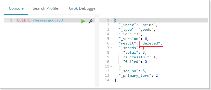
1.8.删除数据
删除使用DELETE请求,同样,需要根据id进行删除:
语法
DELETE /索引库名/类型名/id值
示例:
2.查询
我们从4块来讲查询:
- 基本查询
_source过滤- 结果过滤
- 高级查询
- 排序
2.1.基本查询:
基本语法
GET /索引库名/_search

{

    "query":{

        "查询类型":{

            "查询条件":"查询条件值"

        }

    }

}
这里的query代表一个查询对象,里面可以有不同的查询属性
- 查询类型:
- 例如:
match_all,match,term,range等等
- 例如:
- 查询条件:查询条件会根据类型的不同,写法也有差异,后面详细讲解
2.1.1 查询所有(match_all)
示例:
GET /heima/_search

{

    "query":{

        "match_all": {}

    }

}
query:代表查询对象match_all:代表查询所有
结果:
{

  "took": 2,

  "timed_out": false,

  "_shards": {

    "total": 3,

    "successful": 3,

    "skipped": 0,

    "failed": 0

  },

  "hits": {

    "total": 2,

    "max_score": 1,

    "hits": [

      {

        "_index": "heima",

        "_type": "goods",

        "_id": "2",

        "_score": 1,

        "_source": {

          "title": "大米手机",

          "images": "http://image.leyou.com/12479122.jpg",

          "price": 2899

        }

      },

      {

        "_index": "heima",

        "_type": "goods",

        "_id": "r9c1KGMBIhaxtY5rlRKv",

        "_score": 1,

        "_source": {

          "title": "小米手机",

          "images": "http://image.leyou.com/12479122.jpg",

          "price": 2699

        }

      }

    ]

  }

}
- took:查询花费时间,单位是毫秒
- time_out:是否超时
- _shards:分片信息
- hits:搜索结果总览对象
- total:搜索到的总条数
- max_score:所有结果中文档得分的最高分
- hits:搜索结果的文档对象数组,每个元素是一条搜索到的文档信息
- _index:索引库
- _type:文档类型
- _id:文档id
- _score:文档得分
- _source:文档的源数据
2.1.2 匹配查询(match)
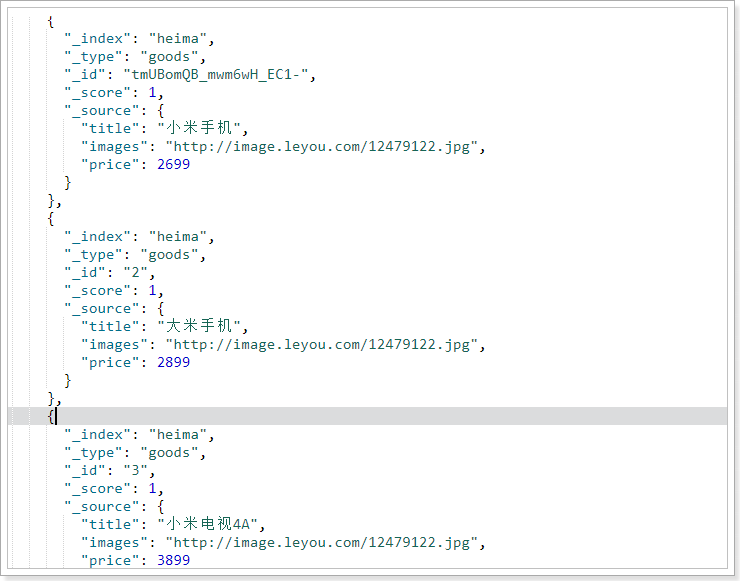
我们先加入一条数据,便于测试:
PUT /heima/goods/3

{

    "title":"小米电视4A",

    "images":"http://image.leyou.com/12479122.jpg",

    "price":3899.00

}
现在,索引库中有2部手机,1台电视:
- or关系
match类型查询,会把查询条件进行分词,然后进行查询,多个词条之间是or的关系
GET /heima/_search

{

    "query":{

        "match":{

            "title":"小米电视"

        }

    }

}
结果:
"hits": {

    "total": 2,

    "max_score": 0.6931472,

    "hits": [

        {

            "_index": "heima",

            "_type": "goods",

            "_id": "tmUBomQB_mwm6wH_EC1-",

            "_score": 0.6931472,

            "_source": {

                "title": "小米手机",

                "images": "http://image.leyou.com/12479122.jpg",

                "price": 2699

            }

        },

        {

            "_index": "heima",

            "_type": "goods",

            "_id": "3",

            "_score": 0.5753642,

            "_source": {

                "title": "小米电视4A",

                "images": "http://image.leyou.com/12479122.jpg",

                "price": 3899

            }

        }

    ]

}
在上面的案例中,不仅会查询到电视,而且与小米相关的都会查询到,多个词之间是or的关系。
- and关系
某些情况下,我们需要更精确查找,我们希望这个关系变成and,可以这样做:
GET /heima/_search

{

    "query":{

        "match": {

          "title": {

            "query": "小米电视",

            "operator": "and"

          }

        }

    }

}
结果:
{

  "took": 2,

  "timed_out": false,

  "_shards": {

    "total": 3,

    "successful": 3,

    "skipped": 0,

    "failed": 0

  },

  "hits": {

    "total": 1,

    "max_score": 0.5753642,

    "hits": [

      {

        "_index": "heima",

        "_type": "goods",

        "_id": "3",

        "_score": 0.5753642,

        "_source": {

          "title": "小米电视4A",

          "images": "http://image.leyou.com/12479122.jpg",

          "price": 3899

        }

      }

    ]

  }

}
本例中,只有同时包含小米和电视的词条才会被搜索到。
- or和and之间?
在 or 与 and 间二选一有点过于非黑即白。 如果用户给定的条件分词后有 5 个查询词项,想查找只包含其中 4 个词的文档,该如何处理?将 operator 操作符参数设置成 and 只会将此文档排除。
有时候这正是我们期望的,但在全文搜索的大多数应用场景下,我们既想包含那些可能相关的文档,同时又排除那些不太相关的。换句话说,我们想要处于中间某种结果。
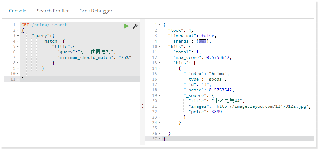
match 查询支持 minimum_should_match 最小匹配参数, 这让我们可以指定必须匹配的词项数用来表示一个文档是否相关。我们可以将其设置为某个具体数字,更常用的做法是将其设置为一个百分数,因为我们无法控制用户搜索时输入的单词数量:
GET /heima/_search

{

    "query":{

        "match":{

            "title":{

            	"query":"小米曲面电视",

            	"minimum_should_match": "75%"

            }

        }

    }

}
本例中,搜索语句可以分为3个词,如果使用and关系,需要同时满足3个词才会被搜索到。这里我们采用最小品牌数:75%,那么也就是说只要匹配到总词条数量的75%即可,这里3*75% 约等于2。所以只要包含2个词条就算满足条件了。
结果:
2.1.3 多字段查询(multi_match)
multi_match与match类似,不同的是它可以在多个字段中查询
GET /heima/_search

{

    "query":{

        "multi_match": {

            "query":    "小米",

            "fields":   [ "title", "subTitle" ]

        }

	}

}
本例中,我们会在title字段和subtitle字段中查询小米这个词
2.1.4 词条匹配(term)
term 查询被用于精确值 匹配,这些精确值可能是数字、时间、布尔或者那些未分词的字符串
GET /heima/_search

{

    "query":{

        "term":{

            "price":2699.00

        }

    }

}
结果:
{

  "took": 2,

  "timed_out": false,

  "_shards": {

    "total": 3,

    "successful": 3,

    "skipped": 0,

    "failed": 0

  },

  "hits": {

    "total": 1,

    "max_score": 1,

    "hits": [

      {

        "_index": "heima",

        "_type": "goods",

        "_id": "r9c1KGMBIhaxtY5rlRKv",

        "_score": 1,

        "_source": {

          "title": "小米手机",

          "images": "http://image.leyou.com/12479122.jpg",

          "price": 2699

        }

      }

    ]

  }

}
2.1.5 多词条精确匹配(terms)
terms 查询和 term 查询一样,但它允许你指定多值进行匹配。如果这个字段包含了指定值中的任何一个值,那么这个文档满足条件:
GET /heima/_search

{

    "query":{

        "terms":{

            "price":[2699.00,2899.00,3899.00]

        }

    }

}
结果:
{

  "took": 4,

  "timed_out": false,

  "_shards": {

    "total": 3,

    "successful": 3,

    "skipped": 0,

    "failed": 0

  },

  "hits": {

    "total": 3,

    "max_score": 1,

    "hits": [

      {

        "_index": "heima",

        "_type": "goods",

        "_id": "2",

        "_score": 1,

        "_source": {

          "title": "大米手机",

          "images": "http://image.leyou.com/12479122.jpg",

          "price": 2899

        }

      },

      {

        "_index": "heima",

        "_type": "goods",

        "_id": "r9c1KGMBIhaxtY5rlRKv",

        "_score": 1,

        "_source": {

          "title": "小米手机",

          "images": "http://image.leyou.com/12479122.jpg",

          "price": 2699

        }

      },

      {

        "_index": "heima",

        "_type": "goods",

        "_id": "3",

        "_score": 1,

        "_source": {

          "title": "小米电视4A",

          "images": "http://image.leyou.com/12479122.jpg",

          "price": 3899

        }

      }

    ]

  }

}
2.2.结果过滤
默认情况下,elasticsearch在搜索的结果中,会把文档中保存在_source的所有字段都返回。
如果我们只想获取其中的部分字段,我们可以添加_source的过滤
2.2.1.直接指定字段
示例:
GET /heima/_search

{

  "_source": ["title","price"],

  "query": {

    "term": {

      "price": 2699

    }

  }

}
返回的结果:
{

  "took": 12,

  "timed_out": false,

  "_shards": {

    "total": 3,

    "successful": 3,

    "skipped": 0,

    "failed": 0

  },

  "hits": {

    "total": 1,

    "max_score": 1,

    "hits": [

      {

        "_index": "heima",

        "_type": "goods",

        "_id": "r9c1KGMBIhaxtY5rlRKv",

        "_score": 1,

        "_source": {

          "price": 2699,

          "title": "小米手机"

        }

      }

    ]

  }

}
2.2.2.指定includes和excludes
我们也可以通过:
- includes:来指定想要显示的字段
- excludes:来指定不想要显示的字段
二者都是可选的。
示例:
GET /heima/_search

{

  "_source": {

    "includes":["title","price"]

  },

  "query": {

    "term": {

      "price": 2699

    }

  }

}
与下面的结果将是一样的:
GET /heima/_search

{

  "_source": {

     "excludes": ["images"]

  },

  "query": {

    "term": {

      "price": 2699

    }

  }

}
2.3 高级查询
2.3.1 布尔组合(bool)
bool把各种其它查询通过must(与)、must_not(非)、should(或)的方式进行组合
GET /heima/_search

{

    "query":{

        "bool":{

        	"must":     { "match": { "title": "大米" }},

        	"must_not": { "match": { "title":  "电视" }},

        	"should":   { "match": { "title": "手机" }}

        }

    }

}
结果:
{

  "took": 10,

  "timed_out": false,

  "_shards": {

    "total": 3,

    "successful": 3,

    "skipped": 0,

    "failed": 0

  },

  "hits": {

    "total": 1,

    "max_score": 0.5753642,

    "hits": [

      {

        "_index": "heima",

        "_type": "goods",

        "_id": "2",

        "_score": 0.5753642,

        "_source": {

          "title": "大米手机",

          "images": "http://image.leyou.com/12479122.jpg",

          "price": 2899

        }

      }

    ]

  }

}
2.3.2 范围查询(range)
range 查询找出那些落在指定区间内的数字或者时间
GET /heima/_search

{

    "query":{

        "range": {

            "price": {

                "gte":  1000.0,

                "lt":   2800.00

            }

    	}

    }

}
range查询允许以下字符:
| 操作符 | 说明 |
|---|---|
| gt | 大于 |
| gte | 大于等于 |
| lt | 小于 |
| lte | 小于等于 |
2.3.3 模糊查询(fuzzy)
我们新增一个商品:
POST /heima/goods/4

{

    "title":"apple手机",

    "images":"http://image.leyou.com/12479122.jpg",

    "price":6899.00

}
fuzzy 查询是 term 查询的模糊等价。它允许用户搜索词条与实际词条的拼写出现偏差,但是偏差的编辑距离不得超过2:
GET /heima/_search

{

  "query": {

    "fuzzy": {

      "title": "appla"

    }

  }

}
上面的查询,也能查询到apple手机
我们可以通过fuzziness来指定允许的编辑距离:
GET /heima/_search

{

  "query": {

    "fuzzy": {

        "title": {

            "value":"appla",

            "fuzziness":1

        }

    }

  }

}
2.4 过滤(filter)
条件查询中进行过滤
所有的查询都会影响到文档的评分及排名。如果我们需要在查询结果中进行过滤,并且不希望过滤条件影响评分,那么就不要把过滤条件作为查询条件来用。而是使用filter方式:
GET /heima/_search

{

    "query":{

        "bool":{

        	"must":{ "match": { "title": "小米手机" }},

        	"filter":{

                "range":{"price":{"gt":2000.00,"lt":3800.00}}

        	}

        }

    }

}
注意:filter中还可以再次进行bool组合条件过滤。
无查询条件,直接过滤
如果一次查询只有过滤,没有查询条件,不希望进行评分,我们可以使用constant_score取代只有 filter 语句的 bool 查询。在性能上是完全相同的,但对于提高查询简洁性和清晰度有很大帮助。
GET /heima/_search

{

    "query":{

        "constant_score":   {

            "filter": {

            	 "range":{"price":{"gt":2000.00,"lt":3000.00}}

            }

        }

}
2.5 排序
2.5.1 单字段排序
sort 可以让我们按照不同的字段进行排序,并且通过order指定排序的方式
GET /heima/_search

{

  "query": {

    "match": {

      "title": "小米手机"

    }

  },

  "sort": [

    {

      "price": {

        "order": "desc"

      }

    }

  ]

}
2.5.2 多字段排序
假定我们想要结合使用 price和 _score(得分) 进行查询,并且匹配的结果首先按照价格排序,然后按照相关性得分排序:
GET /goods/_search

{

    "query":{

        "bool":{

        	"must":{ "match": { "title": "小米手机" }},

        	"filter":{

                "range":{"price":{"gt":200000,"lt":300000}}

        	}

        }

    },

    "sort": [

      { "price": { "order": "desc" }},

      { "_score": { "order": "desc" }}

    ]

}
3. 聚合aggregations
聚合可以让我们极其方便的实现对数据的统计、分析。例如:
- 什么品牌的手机最受欢迎?
- 这些手机的平均价格、最高价格、最低价格?
- 这些手机每月的销售情况如何?
实现这些统计功能的比数据库的sql要方便的多,而且查询速度非常快,可以实现实时搜索效果。
3.1 基本概念
Elasticsearch中的聚合,包含多种类型,最常用的两种,一个叫桶,一个叫度量:
桶(bucket)
桶的作用,是按照某种方式对数据进行分组,每一组数据在ES中称为一个桶,例如我们根据国籍对人划分,可以得到中国桶、英国桶,日本桶……或者我们按照年龄段对人进行划分:010,1020,2030,3040等。
Elasticsearch中提供的划分桶的方式有很多:
- Date Histogram Aggregation:根据日期阶梯分组,例如给定阶梯为周,会自动每周分为一组
- Histogram Aggregation:根据数值阶梯分组,与日期类似
- Terms Aggregation:根据词条内容分组,词条内容完全匹配的为一组
- Range Aggregation:数值和日期的范围分组,指定开始和结束,然后按段分组
- ……
综上所述,我们发现bucket aggregations 只负责对数据进行分组,并不进行计算,因此往往bucket中往往会嵌套另一种聚合:metrics aggregations即度量
度量(metrics)
分组完成以后,我们一般会对组中的数据进行聚合运算,例如求平均值、最大、最小、求和等,这些在ES中称为度量
比较常用的一些度量聚合方式:
- Avg Aggregation:求平均值
- Max Aggregation:求最大值
- Min Aggregation:求最小值
- Percentiles Aggregation:求百分比
- Stats Aggregation:同时返回avg、max、min、sum、count等
- Sum Aggregation:求和
- Top hits Aggregation:求前几
- Value Count Aggregation:求总数
- ……
为了测试聚合,我们先批量导入一些数据
创建索引:
PUT /cars

{

  "settings": {

    "number_of_shards": 1,

    "number_of_replicas": 0

  },

  "mappings": {

    "transactions": {

      "properties": {

        "color": {

          "type": "keyword"

        },

        "make": {

          "type": "keyword"

        }

      }

    }

  }

}
注意:在ES中,需要进行聚合、排序、过滤的字段其处理方式比较特殊,因此不能被分词。这里我们将color和make这两个文字类型的字段设置为keyword类型,这个类型不会被分词,将来就可以参与聚合
导入数据
POST /cars/transactions/_bulk

{ "index": {}}

{ "price" : 10000, "color" : "red", "make" : "honda", "sold" : "2014-10-28" }

{ "index": {}}

{ "price" : 20000, "color" : "red", "make" : "honda", "sold" : "2014-11-05" }

{ "index": {}}

{ "price" : 30000, "color" : "green", "make" : "ford", "sold" : "2014-05-18" }

{ "index": {}}

{ "price" : 15000, "color" : "blue", "make" : "toyota", "sold" : "2014-07-02" }

{ "index": {}}

{ "price" : 12000, "color" : "green", "make" : "toyota", "sold" : "2014-08-19" }

{ "index": {}}

{ "price" : 20000, "color" : "red", "make" : "honda", "sold" : "2014-11-05" }

{ "index": {}}

{ "price" : 80000, "color" : "red", "make" : "bmw", "sold" : "2014-01-01" }

{ "index": {}}

{ "price" : 25000, "color" : "blue", "make" : "ford", "sold" : "2014-02-12" }
3.2 聚合为桶
首先,我们按照 汽车的颜色color来划分桶
GET /cars/_search

{

    "size" : 0,

    "aggs" : {

        "popular_colors" : {

            "terms" : {

              "field" : "color"

            }

        }

    }

}
- size: 查询条数,这里设置为0,因为我们不关心搜索到的数据,只关心聚合结果,提高效率
- aggs:声明这是一个聚合查询,是aggregations的缩写
- popular_colors:给这次聚合起一个名字,任意。
- terms:划分桶的方式,这里是根据词条划分
- field:划分桶的字段
- terms:划分桶的方式,这里是根据词条划分
- popular_colors:给这次聚合起一个名字,任意。
结果:
{

  "took": 1,

  "timed_out": false,

  "_shards": {

    "total": 1,

    "successful": 1,

    "skipped": 0,

    "failed": 0

  },

  "hits": {

    "total": 8,

    "max_score": 0,

    "hits": []

  },

  "aggregations": {

    "popular_colors": {

      "doc_count_error_upper_bound": 0,

      "sum_other_doc_count": 0,

      "buckets": [

        {

          "key": "red",

          "doc_count": 4

        },

        {

          "key": "blue",

          "doc_count": 2

        },

        {

          "key": "green",

          "doc_count": 2

        }

      ]

    }

  }

}
- hits:查询结果为空,因为我们设置了size为0
- aggregations:聚合的结果
- popular_colors:我们定义的聚合名称
- buckets:查找到的桶,每个不同的color字段值都会形成一个桶
- key:这个桶对应的color字段的值
- doc_count:这个桶中的文档数量
通过聚合的结果我们发现,目前红色的小车比较畅销!
3.3 桶内度量
前面的例子告诉我们每个桶里面的文档数量,这很有用。 但通常,我们的应用需要提供更复杂的文档度量。 例如,每种颜色汽车的平均价格是多少?
因此,我们需要告诉Elasticsearch使用哪个字段,使用何种度量方式进行运算,这些信息要嵌套在桶内,度量的运算会基于桶内的文档进行
现在,我们为刚刚的聚合结果添加 求价格平均值的度量:
GET /cars/_search

{

    "size" : 0,

    "aggs" : {

        "popular_colors" : {

            "terms" : {

              "field" : "color"

            },

            "aggs":{

                "avg_price": {

                   "avg": {

                      "field": "price"

                   }

                }

            }

        }

    }

}
- aggs:我们在上一个aggs(popular_colors)中添加新的aggs。可见
度量也是一个聚合,度量是在桶内的聚合 - avg_price:聚合的名称
- avg:度量的类型,这里是求平均值
- field:度量运算的字段
结果:
...

  "aggregations": {

    "popular_colors": {

      "doc_count_error_upper_bound": 0,

      "sum_other_doc_count": 0,

      "buckets": [

        {

          "key": "red",

          "doc_count": 4,

          "avg_price": {

            "value": 32500

          }

        },

        {

          "key": "blue",

          "doc_count": 2,

          "avg_price": {

            "value": 20000

          }

        },

        {

          "key": "green",

          "doc_count": 2,

          "avg_price": {

            "value": 21000

          }

        }

      ]

    }

  }

...
可以看到每个桶中都有自己的avg_price字段,这是度量聚合的结果
3.4 桶内嵌套桶
刚刚的案例中,我们在桶内嵌套度量运算。事实上桶不仅可以嵌套运算, 还可以再嵌套其它桶。也就是说在每个分组中,再分更多组。
比如:我们想统计每种颜色的汽车中,分别属于哪个制造商,按照make字段再进行分桶
GET /cars/_search

{

    "size" : 0,

    "aggs" : {

        "popular_colors" : {

            "terms" : {

              "field" : "color"

            },

            "aggs":{

                "avg_price": {

                   "avg": {

                      "field": "price"

                   }

                },

                "maker":{

                    "terms":{

                        "field":"make"

                    }

                }

            }

        }

    }

}
- 原来的color桶和avg计算我们不变
- maker:在嵌套的aggs下新添一个桶,叫做maker
- terms:桶的划分类型依然是词条
- filed:这里根据make字段进行划分
部分结果:
...

{"aggregations": {

    "popular_colors": {

      "doc_count_error_upper_bound": 0,

      "sum_other_doc_count": 0,

      "buckets": [

        {

          "key": "red",

          "doc_count": 4,

          "maker": {

            "doc_count_error_upper_bound": 0,

            "sum_other_doc_count": 0,

            "buckets": [

              {

                "key": "honda",

                "doc_count": 3

              },

              {

                "key": "bmw",

                "doc_count": 1

              }

            ]

          },

          "avg_price": {

            "value": 32500

          }

        },

        {

          "key": "blue",

          "doc_count": 2,

          "maker": {

            "doc_count_error_upper_bound": 0,

            "sum_other_doc_count": 0,

            "buckets": [

              {

                "key": "ford",

                "doc_count": 1

              },

              {

                "key": "toyota",

                "doc_count": 1

              }

            ]

          },

          "avg_price": {

            "value": 20000

          }

        },

        {

          "key": "green",

          "doc_count": 2,

          "maker": {

            "doc_count_error_upper_bound": 0,

            "sum_other_doc_count": 0,

            "buckets": [

              {

                "key": "ford",

                "doc_count": 1

              },

              {

                "key": "toyota",

                "doc_count": 1

              }

            ]

          },

          "avg_price": {

            "value": 21000

          }

        }

      ]

    }

  }

}

...
- 我们可以看到,新的聚合
maker被嵌套在原来每一个color的桶中。 - 每个颜色下面都根据
make字段进行了分组 - 我们能读取到的信息:
- 红色车共有4辆
- 红色车的平均售价是 $32,500 美元。
- 其中3辆是 Honda 本田制造,1辆是 BMW 宝马制造。
3.5.划分桶的其它方式
前面讲了,划分桶的方式有很多,例如:
- Date Histogram Aggregation:根据日期阶梯分组,例如给定阶梯为周,会自动每周分为一组
- Histogram Aggregation:根据数值阶梯分组,与日期类似
- Terms Aggregation:根据词条内容分组,词条内容完全匹配的为一组
- Range Aggregation:数值和日期的范围分组,指定开始和结束,然后按段分组
刚刚的案例中,我们采用的是Terms Aggregation,即根据词条划分桶。
接下来,我们再学习几个比较实用的:
3.5.1.阶梯分桶Histogram
原理:
histogram是把数值类型的字段,按照一定的阶梯大小进行分组。你需要指定一个阶梯值(interval)来划分阶梯大小。
举例:
比如你有价格字段,如果你设定interval的值为200,那么阶梯就会是这样的:
0,200,400,600,...
上面列出的是每个阶梯的key,也是区间的启点。
如果一件商品的价格是450,会落入哪个阶梯区间呢?计算公式如下:
bucket_key = Math.floor((value - offset) / interval) * interval + offset
value:就是当前数据的值,本例中是450
offset:起始偏移量,默认为0
interval:阶梯间隔,比如200
因此你得到的key = Math.floor((450 - 0) / 200) * 200 + 0 = 400
操作一下:
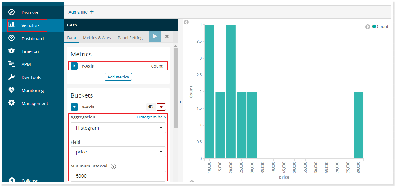
比如,我们对汽车的价格进行分组,指定间隔interval为5000:
GET /cars/_search

{

  "size":0,

  "aggs":{

    "price":{

      "histogram": {

        "field": "price",

        "interval": 5000

      }

    }

  }

}
结果:
{

  "took": 21,

  "timed_out": false,

  "_shards": {

    "total": 5,

    "successful": 5,

    "skipped": 0,

    "failed": 0

  },

  "hits": {

    "total": 8,

    "max_score": 0,

    "hits": []

  },

  "aggregations": {

    "price": {

      "buckets": [

        {

          "key": 10000,

          "doc_count": 2

        },

        {

          "key": 15000,

          "doc_count": 1

        },

        {

          "key": 20000,

          "doc_count": 2

        },

        {

          "key": 25000,

          "doc_count": 1

        },

        {

          "key": 30000,

          "doc_count": 1

        },

        {

          "key": 35000,

          "doc_count": 0

        },

        {

          "key": 40000,

          "doc_count": 0

        },

        {

          "key": 45000,

          "doc_count": 0

        },

        {

          "key": 50000,

          "doc_count": 0

        },

        {

          "key": 55000,

          "doc_count": 0

        },

        {

          "key": 60000,

          "doc_count": 0

        },

        {

          "key": 65000,

          "doc_count": 0

        },

        {

          "key": 70000,

          "doc_count": 0

        },

        {

          "key": 75000,

          "doc_count": 0

        },

        {

          "key": 80000,

          "doc_count": 1

        }

      ]

    }

  }

}
你会发现,中间有大量的文档数量为0 的桶,看起来很丑。
我们可以增加一个参数min_doc_count为1,来约束最少文档数量为1,这样文档数量为0的桶会被过滤
示例:
GET /cars/_search

{

  "size":0,

  "aggs":{

    "price":{

      "histogram": {

        "field": "price",

        "interval": 5000,

        "min_doc_count": 1

      }

    }

  }

}
结果:
{

  "took": 15,

  "timed_out": false,

  "_shards": {

    "total": 5,

    "successful": 5,

    "skipped": 0,

    "failed": 0

  },

  "hits": {

    "total": 8,

    "max_score": 0,

    "hits": []

  },

  "aggregations": {

    "price": {

      "buckets": [

        {

          "key": 10000,

          "doc_count": 2

        },

        {

          "key": 15000,

          "doc_count": 1

        },

        {

          "key": 20000,

          "doc_count": 2

        },

        {

          "key": 25000,

          "doc_count": 1

        },

        {

          "key": 30000,

          "doc_count": 1

        },

        {

          "key": 80000,

          "doc_count": 1

        }

      ]

    }

  }

}
完美,!
如果你用kibana将结果变为柱形图,会更好看:
3.5.2.范围分桶range
范围分桶与阶梯分桶类似,也是把数字按照阶段进行分组,只不过range方式需要你自己指定每一组的起始和结束大小。
最新文章
- 数据结构笔记--二叉查找树概述以及java代码实现
- Hadoop技巧(02):时间同步
- ionic 微信分享值各种坑
- URL编码和解码工具
- lnode满,维护记录
- React Native初试:Windows下Andriod环境搭建
- 上传预览图片自己做的.md
- python sorted用法
- TenxCloud时速云.htaccess不起作用的解决办法
- 开源项目导入eclipse的一般步骤[转]
- Number Sequence ----HDOJ 1711
- hdu5355 Cake(构造)
- Qt学习 之 多线程程序设计(QT通过三种形式提供了对线程的支持)
- 日语编程语言"抚子" - 第三版特色初探
- linux qcom LCD framwork
- keil折叠代码
- “无法将“Enable-Migrations”项识别为 cmdlet、函数、脚本文件或可运行程序的名称。”的一种解决方式
- k8s 1.12.6版的kubeadm默认配置文件
- Codeforces 832C - Strange Radiation
- prometheus监控redis