Morphological Image Processing
Gonzalez R. C. and Woods R. E. Digital Image Processing (Forth Edition)
| 符号 | 即 | 操作 | 说明 |
|---|---|---|---|
| \(\ominus\) | erosion | \(\{z:(B)_z \subset A\}\) | Erodes the boundary of A |
| \(\oplus\) | dilation | \(\{z:(\hat{B})_z \bigcap A \not= \empty\}\) | Dilates the boundary of A |
| \(\circ\) | opening | \((A \ominus B) \oplus B\) | Smoothes contours, breaks narrow isthmuses, and eliminates small islands and sharp peaks. |
| \(\bullet\) | closing | \((A\oplus B) \ominus B\) | Smoothes contours, fuses narrow breaks and long thin gulfs, and eliminates small holes. |
| \(\circledast\) | hit-or-miss | \(\{z:(B)_z \subset I\}\) | Finds I. B contains instances both of foreground B in image and background elements. |
| \(\beta(A)\) | boundary extraction | \(A - (A \ominus B)\) | Set of points on the boundary of set A |
| - | hole filling | \((X_{k-1} \oplus B) \bigcap I^c\) | Fills holes in A |
| - | connected components | \((X_{k-1} \oplus B) \bigcap I\) | Finds connected components in \(I\). |
| \(C(A)\) | convex hull | \((X_{k-1}^i \circledast B^i) \bigcup X_{k-1}^i\) | Finds the convex hull |
| \(\otimes\) | thining | \(A - (A \circledast B)\) | Thins set A |
| \(\odot\) | thickening | \(A\bigcup (A \circledast B)\) | Thickens set A |
| \(S(A)\) | skeleton | $(A \ominus kB) - (A \ominus kB) \circ B $ | Finds the skeleton of set A |
| - | pruning | ... | \(X_4\) is the result of pruning set A. |
| \(D_G^{(1)}(F)\) | geodesic dilation | \((F \oplus B) \bigcap G\) | - |
| \(E_G^{(1)}(F)\) | geodesic erosion | \((F \ominus B) \bigcup G\) | - |
| \(R_G^D(F)\) | morphological reconstruction by dilation | \(R_G^D (F) = D^{(k)}_G (F)\) | - |
| \(R_G^E(F)\) | morphological reconstruction by erosion | \(R_G^E (F) = E^{(k)}_G (F)\) | - |
| \(O_R^{(n)}(F)\) | opening by reconstruction | \(R_{F}^D (F \ominus nB)\) | - |
| \(C_R^{(n)}(F)\) | closing by reconstruction | $ R_{F}^E (F \oplus nB)$ | - |
| - | hole filling | $H = [R_{Ic}D(F)]^c $ | Auto |
| - | border clearing | \(I - R_I^D(F)\) | - |
概
直接把整个章节都拿来是决定这个形态学的东西实在是有趣, 加之前后联系过于紧密, 感觉如果过于割裂会导致以后回忆不起来, 所以直接对整个章节做个笔记得了.
我觉得首先需要牢记的是, 本章节是在集合的基础上讨论的, 对于一个二元图中的物体, 我们可以通过如下集合表示:
\]
\((x, y)\)表示值为\(1\)的坐标(这里假设foreground pixel的值为1, 当然也可以假设其为0).
注: 个人觉得, 这里讨论的时候并非像之前的图片一样以左上角原点, 而是以目标中心为原点然后发散开去(只是单纯便于理解和书写, 实际处理是不受影响的). 也就意味着, \(x, y\)是可以为负的, 显然这种表示的好处是不需要确定整个图片的大小范围.
本章节会频繁涉及到objects和structuring elements (SE)的概念, 说实话其具体的定义不是很清楚, 我还是从任务的角度来给它们做个解释.
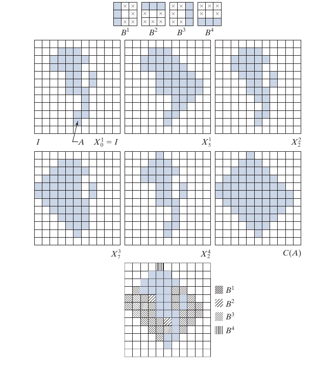
因为本章节讨论的transform, 通常都是通过SE经过一些集合操作使得objects发生某种改变, 所以objects就是对象. SE
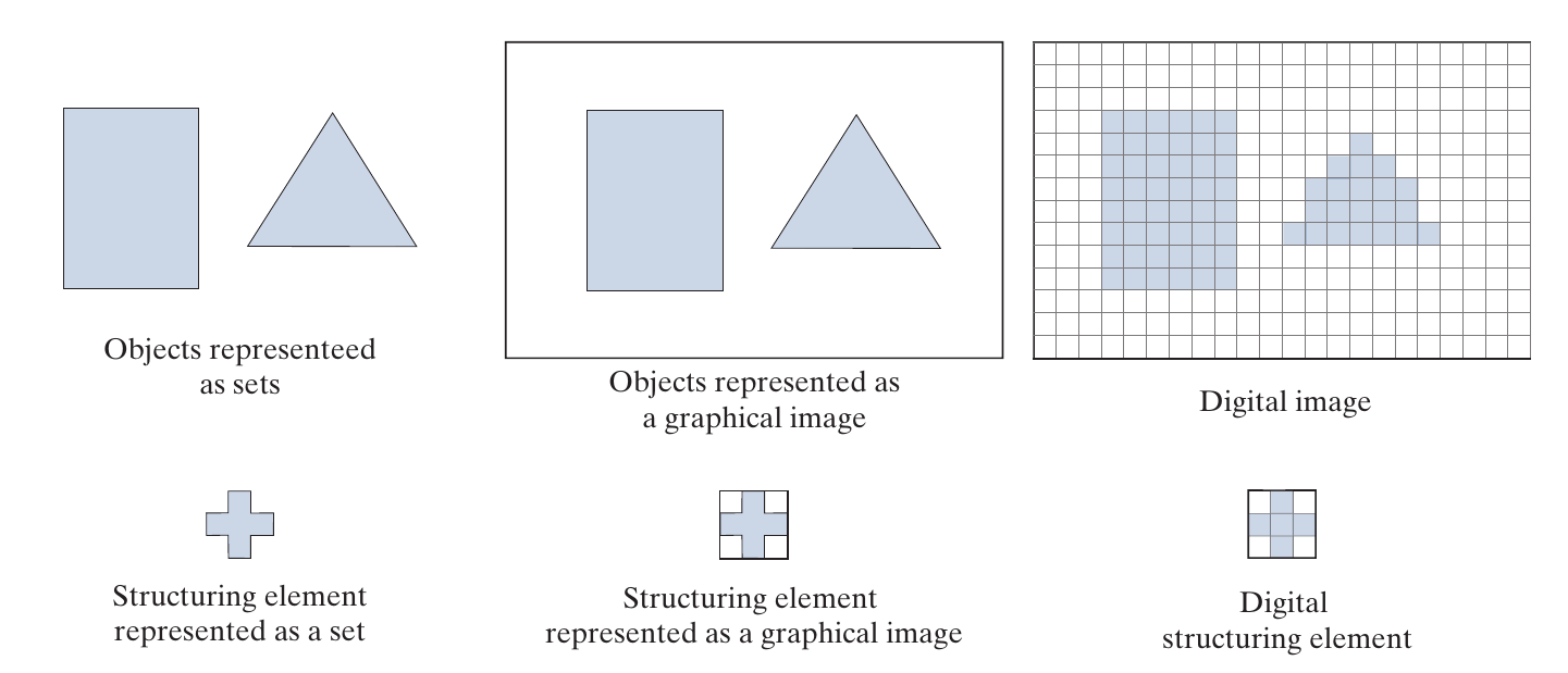
如上图所示, 虽然objects是一个仅仅记录0值的集合, 我们通常将其置于一个矩形区域中, 便于图片的处理, SE也是类似的. 特别的是, SE整体除了0, 1外还可能有\(\times\)的属性, 其表示0或1, 即该位置的点不我们所关心的点, 其可以任意匹配.
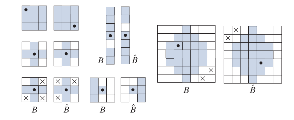
reflection and translation
反射, 即
\]
需要注意的是该反射是以\(B\)的中心为原点的.
平移, 即
\]
Erosion and Dilation
Erosion
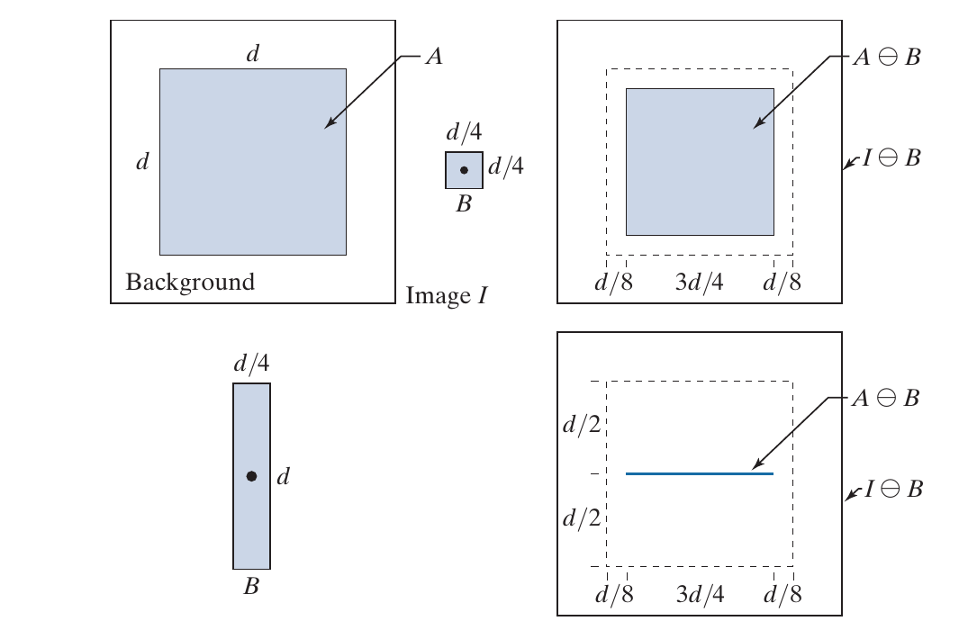
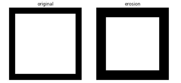
Erosion操作能够令图片中的元素'缩小', 所以其在处理噪声的时候其实不错. 其定义为:
A \ominus B &= \{z| (B)_z \subset A\} \\
&= \{w \in Z^2 | w + b \in A \text{ for every } b \in B\} \\
&= \mathop{\bigcap} \limits_{b \in B} (A)_{-b}.
\end{array}
\]
proof:
设上面三个定义分别为\(C_1, C_2, C_3\).
\(C_1 \subset C_2\):
\(\forall z \in C_1\),
\]
故
\]
\(C_2 = C_3\):
=\bigcap_{b \in B} \{a-b \in Z^2 | \in A\}
=\bigcap_{b \in B} (A)_{-b}.
\]
\(C_3 \subset C_1\):
\(\forall w \in C_2\):
\]
示例
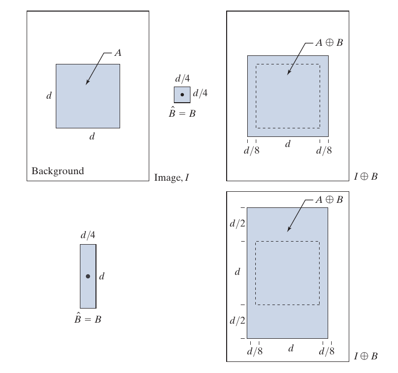
如下图所示, 第一行第一幅图是object, 通过第二幅SE erosion后object缩小了, 而通过第二行的SE更是直接成了一条线.
skimage.morphology.erosion
[erosion](Module: morphology — skimage v0.19.0.dev0 docs (scikit-image.org))
import numpy as np

import matplotlib.pyplot as plt

from skimage.morphology import erosion, disk

def plot_comparison(original, filtered, filter_name):

    fig, (ax1, ax2) = plt.subplots(ncols=2, figsize=(8, 4), sharex=True,

                                   sharey=True)

    ax1.imshow(original, cmap=plt.cm.gray)

    ax1.set_title('original')

    ax1.axis('off')

    ax2.imshow(filtered, cmap=plt.cm.gray)

    ax2.set_title(filter_name)

    ax2.axis('off')
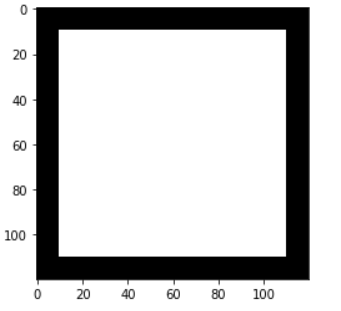
img = np.ones((100, 100))

arow = np.zeros((10, 100))

img = np.vstack((arow, img, arow))

acol = np.zeros((120, 10))

img = np.hstack((acol, img, acol)).astype(np.uint8)

fig, ax = plt.subplots()

ax.imshow(img, cmap=plt.cm.gray)
footprint = disk(6) # {0, 1}, 半径为6的圆, 中心元素为1其余为0

eroded = erosion(img, footprint)

plot_comparison(img, eroded, 'erosion')
dilation
dilation的效果是令图中的元素进行扩张, 一些扫描的文本图像可能字符剑有断痕, 通过此可以修复.
其集合定义为:
A \oplus B
&= \{z| (\hat{B})_z \bigcap A \not= \empty\} \\
&= \{w \in Z^2| w = a+ b, \text{ for some } a \in A \text{ and } b \in B\}\\
&= \mathop{\bigcup}_{b \in B} (A)_b \\
&= \mathop{\bigcup}_{a \in A} (B)_a.
\end{array}
\]
proof:
记上面四种定义各自为\(C_1, C_2, C_3, C_4\):
\(C_1 = C_2\):
\(\forall z \in C_1\):
\]
故
\]
\(\forall w \in C_2\):
\]
故
\]
\(C_2 = C_3 = C_4\):
显然.
最后两个定义是很直观的, \(C_3\)相当于对于每一个点\(b\in B\)为中心画一个\(A\), \(C_4\)则是以每一个\(a \in A\)为中心画一个\(B\).
示例
skimage.morphology.dilation
from skimage.morphology import dilation

footprint = disk(6) # {0, 1}, 半径为6的圆, 中心元素为1其余为0

dilated = dilation(eroded, footprint)

plot_comparison(eroded, dilated, 'dilation')
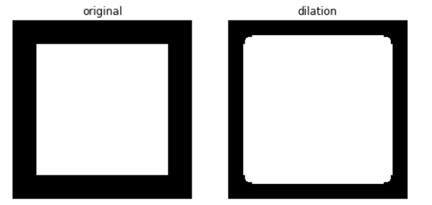
注: 圆角实际上是下一节的东西.
对偶性
(A\ominus B)^c
&= \{z| (B)_z \subset A\}^c \\
&= \{z| (B)_z \bigcap A^c \not = \empty\} \\
&= A^c \oplus \hat{B}.
\end{array}
\]
(A\oplus B)^c
&= \{z| (\hat{B})_z \bigcap A \not= \empty \}^c \\
&= \{z| (\hat{B})_z \subset A^c\} \\
&= A^c \ominus \hat{B}.
\end{array}
\]
Opening and Closing
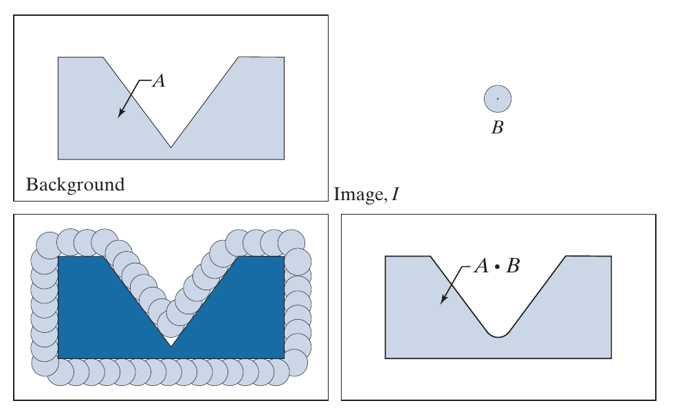
二者都有一种将目标变圆滑的效果.
Opening
定义:
\]
proof:
(A \ominus B) \oplus B
&= \bigcup_{z \in A \ominus B} (B)_z \\
&= \bigcup_{z} \{(B)_z| (B)_z \subset A\}.
\end{array}
\]
示例

skimage.morphology.opening
from skimage.morphology import opening

footprint = disk(6)

opened = opening(img, footprint)

plot_comparison(img, opened, 'opening')

Closing
定义:
\]
注: 书中为:
\]
但感觉不一样啊.
proof:
[(A \oplus B) \ominus B]^c
&= (A \oplus B)^c \oplus \hat{B} \\
&= (A^c \ominus \hat{B}) \oplus \hat{B} \\
&= \bigcup_z \{(\hat{B})_z | (\hat{B})_z \subset A^c\} \\
&= \bigcup_z \{(\hat{B})_z | (\hat{B})_z \bigcap A = \empty\} \\
\end{array}
\]
示例
skimage.morphology.closing
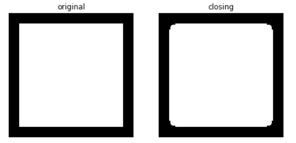
from skimage.morphology import closing

footprint = disk(6)

closed = opening(img, footprint)

plot_comparison(img, closed, 'closing')
对偶性
(A \bullet B)^c = (A^c \circ \hat{B})
\]
且
(A \bullet B) \bullet B = A \bullet B.
\]
The Hit-or-Miss Transform
主要用于shape detection.
定义:
\]
此为\(B_1, B_2\)不包含\(0\)元素的情形, 倘若允许\(B\)包含0元素, 那么
\]
只是我们\(B\)通常需要一些特殊的性质来使其具有detection的作用.
具体怎么shape detection 还是请回看原文吧.
一些基本的操作
Boundary Extraction
定义:
\]
直观的感觉就是把object的中间部分挖掉.
Hole Filling
假设在我们想填的hole中已知一个点, 以这个点为基础出发(记为\(X_0\)):
\]
停止准则为
\]
不过需要注意的是, \(B\)应该选择下面类型的(如果是全满的话可能跳出hole了).
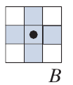
Extraction of Connected Components
抓取连通区域, 假设已知在我们想抓取的连通区域的一点, 从这个点出发(记为\(X_0\)):
\]
直到
\]
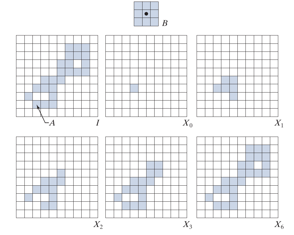
Convex Hull
将一个object填补成凸的, 这个说实话没怎么看明白.
X_0^i = I.
\]
当
\]
时停止, 记其为\(D^i\), 最后的convex hull 为
\]
总感觉这个不是最小的凸包啊.
skimage.morphology.convex_hull_image
Thinning
定义:
\]

skimage.morphology.thin
Thickening
相反的操作:
\]

Skeletons
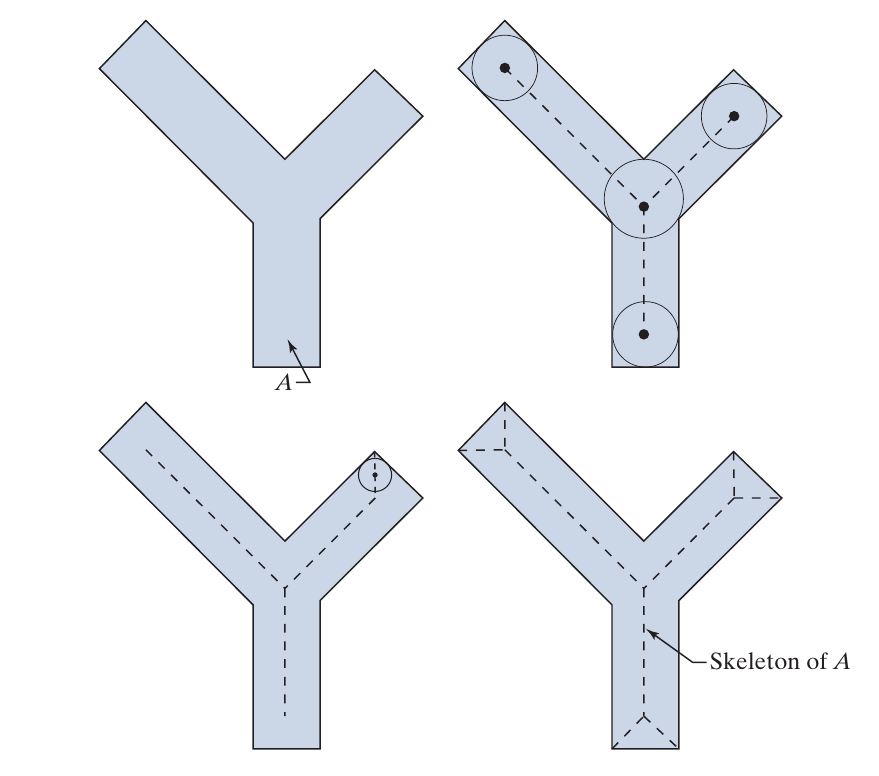
其严格的定义有些复杂, 感觉有点拓扑结构?
S_k(A) = (A \ominus kB) - (A \ominus kB) \circ B \\
(A \ominus kB) = ((\ldots ((A\ominus B) \ominus B)\ominus \ldots) \ominus B)\\
K = \max \{k| (A \ominus kB) \not = \empty \}.
\]
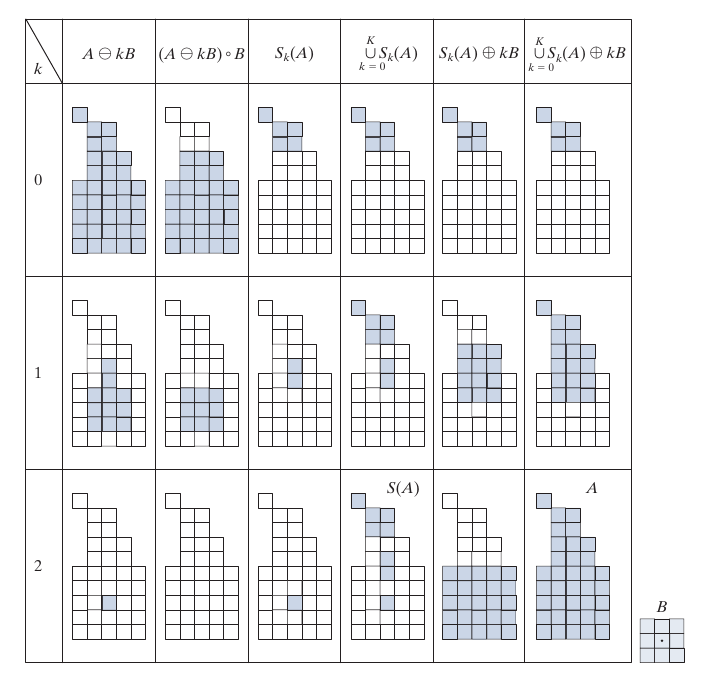
skimage.morphology.skeletonize
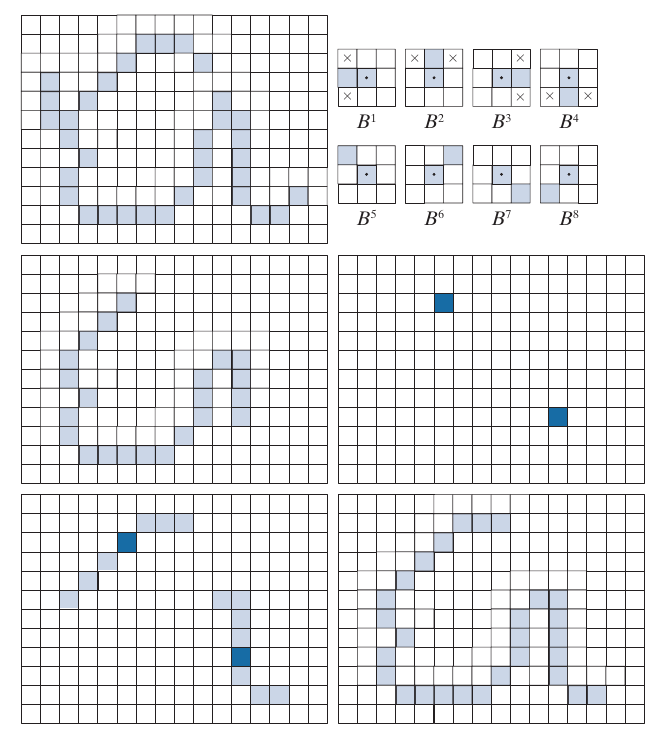
Pruning
pruning 方法用于去掉别的方法留下的一些spurs:
X_2 = \mathop{\bigcup} \limits_{k=1}^8 (X_1 \circledast B^k) \\
X_3 = (X_2 \oplus H) \bigcap A \\
X_4 = X_1 \bigcup X_3.
\]
\(B^k\)为下图的一系列(而\(\{B\}\)为其中一部分不一定全部用到):
Morphological Reconstruction
Morphological Reconstruction除了之前用到的\(F, B\)外, 还要额外用到一个图片(称为mask)作为一个reconstruction的limit.
Geodesic Dilation and Erosion
假设\(F \subset G\), geodesic dilation:
D_G^{(n)} (F) = D_G^{(1)} (D_G^{(n-1)} (F)), \quad D_G^{(0)} (F) = F.
\]
geodesic erosion:
E_G^{(n)}(F) = E_G^{(1)}(E_G^{(n-1)}(F)), \quad E_G^{(0)}(F) = F.
\]
直观上很好解释, 即geodesic dilation在扩张的时候不能超过\(G\), 而geodesic erosion在收缩的时候不会少于\(G\).
Morphological Reconstruction by Dilation and by Erosion
定义很简单, 即重复上述操作直到收敛:
R_G^E (F) = E^{(k)}_G (F), \quad \text{if } E^{(k)}_G (F) = E^{(k-1)}_G (F).
\]
Opening|Closing by Reconstruction
\]
直观解释就是, 先erosion \(n\)次, 再在此基础上不断扩张(受限于\(F\)).
Closing by Reconstruction 就是:
\]

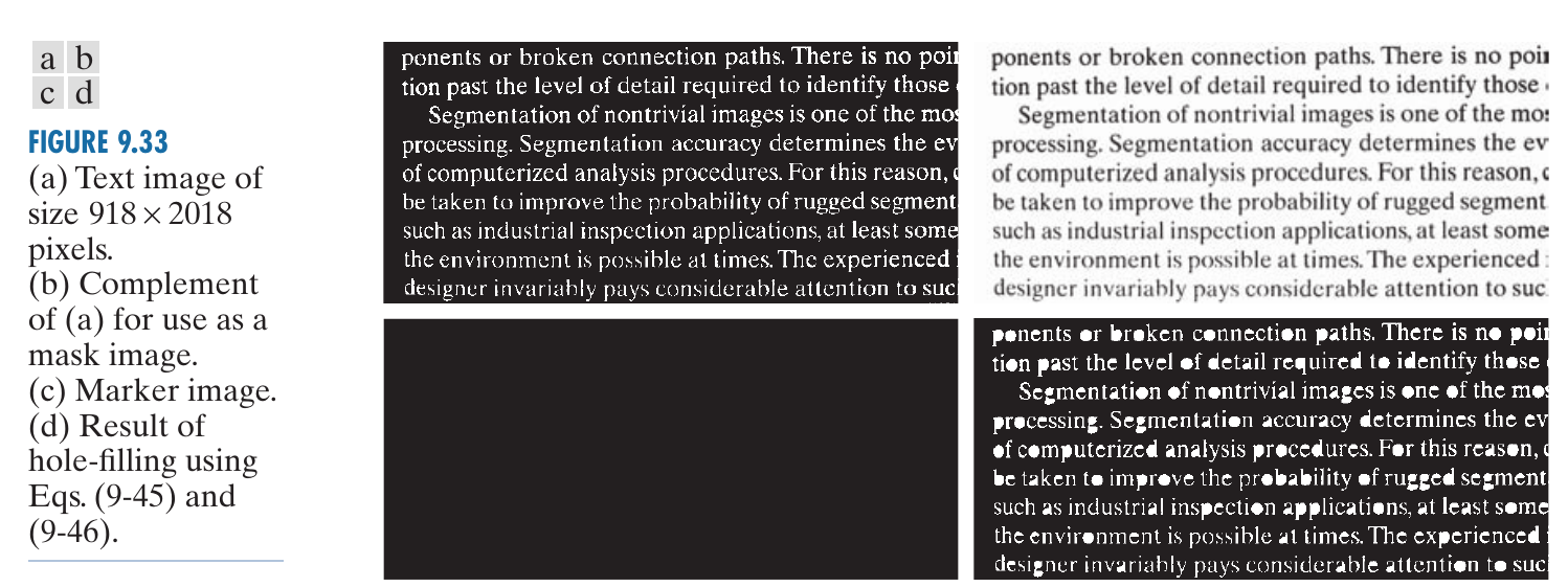
Automatic Algorithm for Filling Holes
之前介绍的hole filling需要一个点为基础, 这个算法是全自动的.
\left \{
\begin{array}{ll}
1 - I(x, y) & \text{if } (x, y) \text{ is on the border of } I \\
0 & \text{otherwise}.
\end{array}
\right .
\]
H \bigcap I^c
\]
感觉还是挺好理解的, 就是从边边, 由于中间部分的hole一定会被包围起来, 所以\(H^c\)一定不包含中间部分的hole.
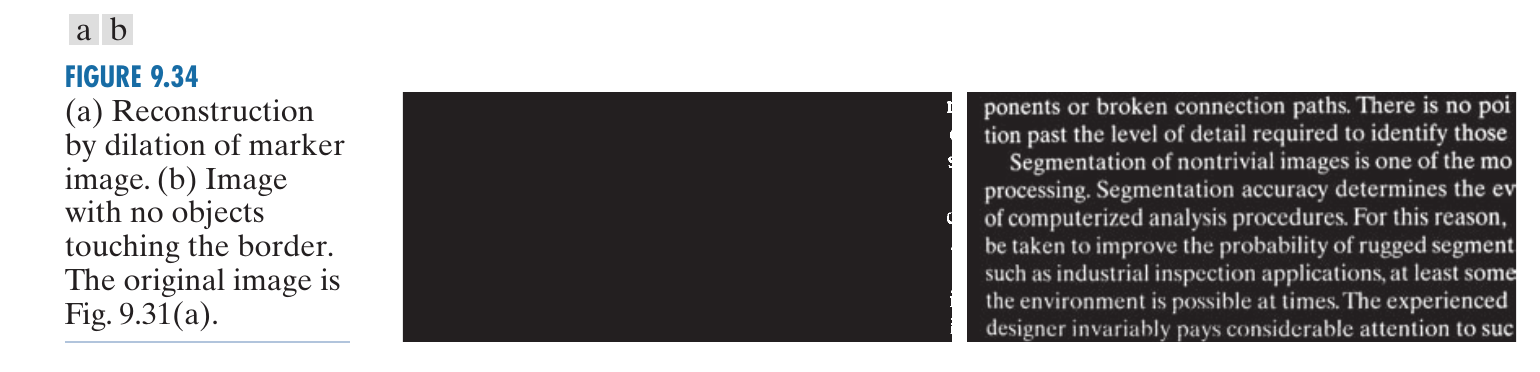
Border Clearing
\left \{
\begin{array}{ll}
I(x, y) & \text{if } (x, y) \text{ is on the border of } I \\
0 & \text{otherwise}.
\end{array}
\right .
\]
\]
能够把边缘的一些部分给去了.
最新文章
- 自己动手编写spring IOC源码
- SSH使用详解
- web前端笔试选择题
- 【linux】linux shell 日期格式化
- iOS 获取设备版本型号
- PHP内存溢出解决方案
- [ruby on rails] 深入(1) ROR的一次request的响应过程
- Linux下对各种压缩文件处理
- c++ 程序在内存中的分布
- Node.js 异步模式浅析
- sublime3运行lua
- AndroidPN中的心跳检测
- 1.23 确定一个Decimal或Double的整数部分
- 关于前端JS模块加载器实现的一些细节
- 根据抽象工厂实现的DBHelpers类
- ES 08 - 创建、查看、修改、删除、关闭Elasticsearch的index
- Could not resolve placeholder 'IMAGE_SERVER_URL' in string value "${IMAGE_SERVER_URL}"
- 用php写一个99乘法表
- .NET并行计算和并发11:并发接口 IProducerConsumerCollection
- [nodejs]er_bad_field_error NaN in where clause