【机器学习】用Octave实现一元线性回归的梯度下降算法
2024-09-30 00:16:36
Step1 Plotting the Data
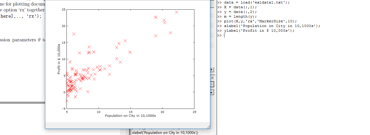
在处理数据之前,我们通常要了解数据,对于这次的数据集合,我们可以通过离散的点来描绘它,在一个2D的平面里把它画出来。
6.1101,17.592

5.5277,9.1302

8.5186,13.662

7.0032,11.854

5.8598,6.8233

8.3829,11.886

7.4764,4.3483

8.5781,12

6.4862,6.5987

5.0546,3.8166

5.7107,3.2522

14.164,15.505

5.734,3.1551

8.4084,7.2258

5.6407,0.71618

5.3794,3.5129

6.3654,5.3048

5.1301,0.56077

6.4296,3.6518

7.0708,5.3893

6.1891,3.1386

20.27,21.767

5.4901,4.263

6.3261,5.1875

5.5649,3.0825

18.945,22.638

12.828,13.501

10.957,7.0467

13.176,14.692

22.203,24.147

5.2524,-1.22

6.5894,5.9966

9.2482,12.134

5.8918,1.8495

8.2111,6.5426

7.9334,4.5623

8.0959,4.1164

5.6063,3.3928

12.836,10.117

6.3534,5.4974

5.4069,0.55657

6.8825,3.9115

11.708,5.3854

5.7737,2.4406

7.8247,6.7318

7.0931,1.0463

5.0702,5.1337

5.8014,1.844

11.7,8.0043

5.5416,1.0179

7.5402,6.7504

5.3077,1.8396

7.4239,4.2885

7.6031,4.9981

6.3328,1.4233

6.3589,-1.4211

6.2742,2.4756

5.6397,4.6042

9.3102,3.9624

9.4536,5.4141

8.8254,5.1694

5.1793,-0.74279

21.279,17.929

14.908,12.054

18.959,17.054

7.2182,4.8852

8.2951,5.7442

10.236,7.7754

5.4994,1.0173

20.341,20.992

10.136,6.6799

7.3345,4.0259

6.0062,1.2784

7.2259,3.3411

5.0269,-2.6807

6.5479,0.29678

7.5386,3.8845

5.0365,5.7014

10.274,6.7526

5.1077,2.0576

5.7292,0.47953

5.1884,0.20421

6.3557,0.67861

9.7687,7.5435

6.5159,5.3436

8.5172,4.2415

9.1802,6.7981

6.002,0.92695

5.5204,0.152

5.0594,2.8214

5.7077,1.8451

7.6366,4.2959

5.8707,7.2029

5.3054,1.9869

8.2934,0.14454

13.394,9.0551

5.4369,0.61705
ex1data1.txt
我们把ex1data1中的内容读取到X变量和y变量中,用m表示数据长度。
data = load('ex1data1.txt');

X = data(:,1);

y = data(:,2);

m = length(y);
接下来通过图像描绘出来。
plot(x,y,'rx','MakerSize',10);

ylabel('Profit in $10,000s');

xlabel('Population of City in 10,000s');
现在我们得到图像如图所示,就是原始的数据的直观表示。
Step2 Gradient Descent
现在,我们通过梯度下降法对参数θ进行线性回归。
依照我们之前所得出步骤方法

迭代更新
计算θ值函数:
function J = computeCost(X, y, theta)

%COMPUTECOST Compute cost for linear regression

%   J = COMPUTECOST(X, y, theta) computes the cost of using theta as the

%   parameter for linear regression to fit the data points in X and y

% Initialize some useful values

m = length(y); % number of training examples

% You need to return the following variables correctly

J = 0;

% ====================== YOUR CODE HERE ======================

% Instructions: Compute the cost of a particular choice of theta

%               You should set J to the cost.

J = sum((X * theta - y).^2) / (2*m);     % X(79,2)  theta(2,1)

% =========================================================================

end
接下来是梯度下降函数
function [theta, J_history] = gradientDescent(X, y, theta, alpha, num_iters)

%GRADIENTDESCENT Performs gradient descent to learn theta

%   theta = GRADIENTDESENT(X, y, theta, alpha, num_iters) updates theta by

%   taking num_iters gradient steps with learning rate alpha

% Initialize some useful values

m = length(y); % number of training examples

J_history = zeros(num_iters, 1);

theta_s=theta;

for iter = 1:num_iters

    % ====================== YOUR CODE HERE ======================

    % Instructions: Perform a single gradient step on the parameter vector

    %               theta.

    %

    % Hint: While debugging, it can be useful to print out the values

    %       of the cost function (computeCost) and gradient here.

    %

    theta(1) = theta(1) - alpha / m * sum(X * theta_s - y);

    theta(2) = theta(2) - alpha / m * sum((X * theta_s - y) .* X(:,2));

% 必须同时更新theta(1)和theta(2),所以不能用X * theta,而要用theta_s存储上次结果。

    theta_s=theta;

    % ============================================================

    % Save the cost J in every iteration

    J_history(iter) = computeCost(X, y, theta);

end

J_history

end
绘图函数:
function plotData(x, y)

%PLOTDATA Plots the data points x and y into a new figure

% PLOTDATA(x,y) plots the data points and gives the figure axes labels of

% population and profit.

% ====================== YOUR CODE HERE ======================

% Instructions: Plot the training data into a figure using the

% "figure" and "plot" commands. Set the axes labels using

% the "xlabel" and "ylabel" commands. Assume the

% population and revenue data have been passed in

% as the x and y arguments of this function.

%

% Hint: You can use the 'rx' option with plot to have the markers

% appear as red crosses. Furthermore, you can make the

% markers larger by using plot(..., 'rx', 'MarkerSize', 10);

figure; % open a new figure window

plot(x, y, 'rx', 'MarkerSize', 10); % Plot the data

ylabel('Profit in $10,000s'); % Set the y axis label

xlabel('Population of City in 10,000s'); % Set the x axis label

% ============================================================

end
根据以上函数,我们进行线性回归:
%% Machine Learning Online Class - Exercise 1: Linear Regression

%  Instructions

%  ------------

%

%  This file contains code that helps you get started on the

%  linear exercise. You will need to complete the following functions

%  in this exericse:

%

%     warmUpExercise.m

%     plotData.m

%     gradientDescent.m

%     computeCost.m

%     gradientDescentMulti.m

%     computeCostMulti.m

%     featureNormalize.m

%     normalEqn.m

%

%  For this exercise, you will not need to change any code in this file,

%  or any other files other than those mentioned above.

%

% x refers to the population size in 10,000s

% y refers to the profit in $10,000s

%

%% ==================== Part 1: Basic Function ====================

% Complete warmUpExercise.m

fprintf('Running warmUpExercise ... \n');

fprintf('5x5 Identity Matrix: \n');

warmUpExercise()

fprintf('Program paused. Press enter to continue.\n');

pause;

%% ======================= Part 2: Plotting =======================

fprintf('Plotting Data ...\n')

data = load('ex1data1.txt');

X = data(:, 1); y = data(:, 2);

m = length(y); % number of training examples

% Plot Data

% Note: You have to complete the code in plotData.m

plotData(X, y);

fprintf('Program paused. Press enter to continue.\n');

pause;

%% =================== Part 3: Gradient descent ===================

fprintf('Running Gradient Descent ...\n')

X = [ones(m, 1), data(:,1)]; % Add a column of ones to x

theta = zeros(2, 1); % initialize fitting parameters

% Some gradient descent settings

iterations = 1500;

alpha = 0.01;

% compute and display initial cost

computeCost(X, y, theta)

% run gradient descent

theta = gradientDescent(X, y, theta, alpha, iterations);

% print theta to screen

fprintf('Theta found by gradient descent: ');

fprintf('%f %f \n', theta(1), theta(2));

% Plot the linear fit

hold on; % keep previous plot visible

plot(X(:,2), X*theta, '-')

legend('Training data', 'Linear regression')

hold off % don't overlay any more plots on this figure

% Predict values for population sizes of 35,000 and 70,000

predict1 = [1, 3.5] *theta;

fprintf('For population = 35,000, we predict a profit of %f\n',...

    predict1*10000);

predict2 = [1, 7] * theta;

fprintf('For population = 70,000, we predict a profit of %f\n',...

    predict2*10000);

fprintf('Program paused. Press enter to continue.\n');

pause;

%% ============= Part 4: Visualizing J(theta_0, theta_1) =============

fprintf('Visualizing J(theta_0, theta_1) ...\n')

% Grid over which we will calculate J

theta0_vals = linspace(-10, 10, 100);

theta1_vals = linspace(-1, 4, 100);

% initialize J_vals to a matrix of 0's

J_vals = zeros(length(theta0_vals), length(theta1_vals));

% Fill out J_vals

for i = 1:length(theta0_vals)

    for j = 1:length(theta1_vals)

	  t = [theta0_vals(i); theta1_vals(j)];

	  J_vals(i,j) = computeCost(X, y, t);

    end

end

% Because of the way meshgrids work in the surf command, we need to

% transpose J_vals before calling surf, or else the axes will be flipped

J_vals = J_vals';

% Surface plot

figure;

surf(theta0_vals, theta1_vals, J_vals)

xlabel('\theta_0'); ylabel('\theta_1');

% Contour plot

figure;

% Plot J_vals as 15 contours spaced logarithmically between 0.01 and 100

contour(theta0_vals, theta1_vals, J_vals, logspace(-2, 3, 20))

xlabel('\theta_0'); ylabel('\theta_1');

hold on;

plot(theta(1), theta(2), 'rx', 'MarkerSize', 10, 'LineWidth', 2);

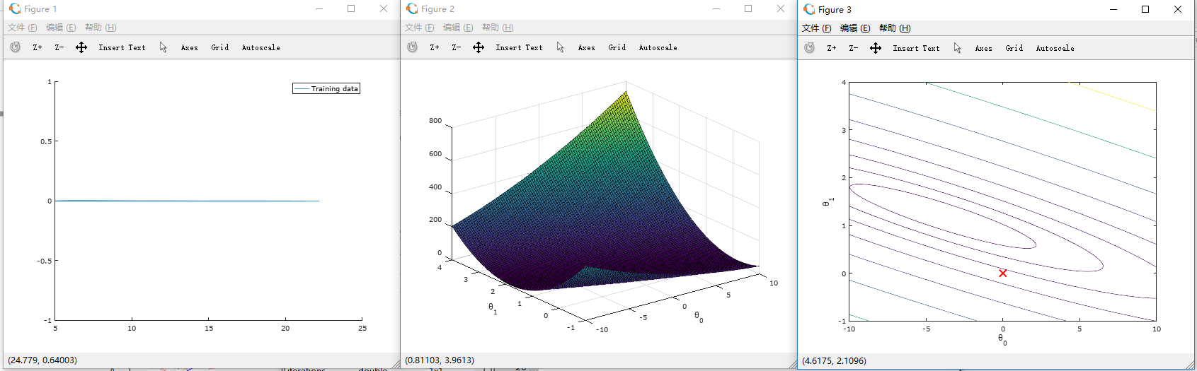
如图所示,绘制出线性回归函数。
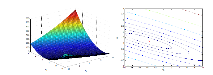
这时所绘制2D等高线图梯度下降表面图:
function [X_norm, mu, sigma] = featureNormalize(X)
%FEATURENORMALIZE Normalizes the features in X
% FEATURENORMALIZE(X) returns a normalized version of X where
% the mean value of each feature is 0 and the standard deviation
% is 1. This is often a good preprocessing step to do when
% working with learning algorithms. % You need to set these values correctly
X_norm = X;
mu = zeros(1, size(X, 2)); % mean value 均值 size(X,2) 列数
sigma = zeros(1, size(X, 2)); % standard deviation 标准差 % ====================== YOUR CODE HERE ======================
% Instructions: First, for each feature dimension, compute the mean
% of the feature and subtract it from the dataset,
% storing the mean value in mu. Next, compute the
% standard deviation of each feature and divide
% each feature by it's standard deviation, storing
% the standard deviation in sigma.
%
% Note that X is a matrix where each column is a
% feature and each row is an example. You need
% to perform the normalization separately for
% each feature.
%
% Hint: You might find the 'mean' and 'std' functions useful.
%
mu = mean(X); % mean value
sigma = std(X); % standard deviation
X_norm = (X - repmat(mu,size(X,1),1)) ./ repmat(sigma,size(X,1),1); % ============================================================ end
function [theta, J_history] = gradientDescentMulti(X, y, theta, alpha, num_iters)
%GRADIENTDESCENTMULTI Performs gradient descent to learn theta
% theta = GRADIENTDESCENTMULTI(x, y, theta, alpha, num_iters) updates theta by
% taking num_iters gradient steps with learning rate alpha % Initialize some useful values
m = length(y); % number of training examples
J_history = zeros(num_iters, 1); for iter = 1:num_iters % ====================== YOUR CODE HERE ======================
% Instructions: Perform a single gradient step on the parameter vector
% theta.
%
% Hint: While debugging, it can be useful to print out the values
% of the cost function (computeCostMulti) and gradient here.
%
theta = theta - alpha / m * X' * (X * theta - y); % ============================================================ % Save the cost J in every iteration
J_history(iter) = computeCostMulti(X, y, theta); end end
function J = computeCostMulti(X, y, theta)
%COMPUTECOSTMULTI Compute cost for linear regression with multiple variables
% J = COMPUTECOSTMULTI(X, y, theta) computes the cost of using theta as the
% parameter for linear regression to fit the data points in X and y % Initialize some useful values
m = length(y); % number of training examples % You need to return the following variables correctly
J = 0; % ====================== YOUR CODE HERE ======================
% Instructions: Compute the cost of a particular choice of theta
% You should set J to the cost.
J = sum((X * theta - y).^2) / (2*m); % ========================================================================= end
function [theta] = normalEqn(X, y)
%NORMALEQN Computes the closed-form solution to linear regression
% NORMALEQN(X,y) computes the closed-form solution to linear
% regression using the normal equations. theta = zeros(size(X, 2), 1); % ====================== YOUR CODE HERE ======================
% Instructions: Complete the code to compute the closed form solution
% to linear regression and put the result in theta.
% % ---------------------- Sample Solution ---------------------- theta = pinv( X' * X ) * X' * y; % ------------------------------------------------------------- % ============================================================ end
%% Machine Learning Online Class
% Exercise 1: Linear regression with multiple variables
%
% Instructions
% ------------
%
% This file contains code that helps you get started on the
% linear regression exercise.
%
% You will need to complete the following functions in this
% exericse:
%
% warmUpExercise.m
% plotData.m
% gradientDescent.m
% computeCost.m
% gradientDescentMulti.m
% computeCostMulti.m
% featureNormalize.m
% normalEqn.m
%
% For this part of the exercise, you will need to change some
% parts of the code below for various experiments (e.g., changing
% learning rates).
% %% Initialization %% ================ Part 1: Feature Normalization ================ %% Clear and Close Figures
clear ; close all; clc fprintf('Loading data ...\n'); %% Load Data
data = load('ex1data2.txt');
X = data(:, 1:2);
y = data(:, 3);
m = length(y); % Print out some data points
fprintf('First 10 examples from the dataset: \n');
fprintf(' x = [%.0f %.0f], y = %.0f \n', [X(1:10,:) y(1:10,:)]'); fprintf('Program paused. Press enter to continue.\n');
pause; % Scale features and set them to zero mean
fprintf('Normalizing Features ...\n'); [X mu sigma] = featureNormalize(X); % 均值0,标准差1 % Add intercept term to X
X = [ones(m, 1) X]; %% ================ Part 2: Gradient Descent ================ % ====================== YOUR CODE HERE ======================
% Instructions: We have provided you with the following starter
% code that runs gradient descent with a particular
% learning rate (alpha).
%
% Your task is to first make sure that your functions -
% computeCost and gradientDescent already work with
% this starter code and support multiple variables.
%
% After that, try running gradient descent with
% different values of alpha and see which one gives
% you the best result.
%
% Finally, you should complete the code at the end
% to predict the price of a 1650 sq-ft, 3 br house.
%
% Hint: By using the 'hold on' command, you can plot multiple
% graphs on the same figure.
%
% Hint: At prediction, make sure you do the same feature normalization.
% fprintf('Running gradient descent ...\n'); % Choose some alpha value
alpha = 0.01;
num_iters = 8500; % Init Theta and Run Gradient Descent
theta = zeros(3, 1);
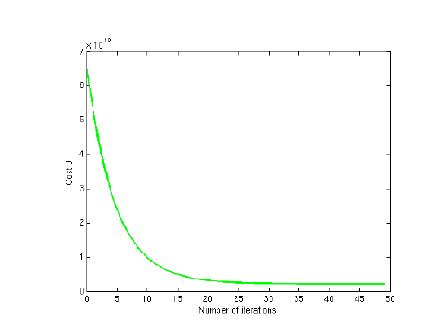
[theta, J_history] = gradientDescentMulti(X, y, theta, alpha, num_iters); % Plot the convergence graph
figure;
plot(1:numel(J_history), J_history, '-b', 'LineWidth', 2);
xlabel('Number of iterations');
ylabel('Cost J'); % Display gradient descent's result
fprintf('Theta computed from gradient descent: \n');
fprintf(' %f \n', theta);
fprintf('\n'); % Estimate the price of a 1650 sq-ft, 3 br house
% ====================== YOUR CODE HERE ======================
% Recall that the first column of X is all-ones. Thus, it does
% not need to be normalized.
price = [1 (([1650 3]-mu) ./ sigma)] * theta ;
% ============================================================ fprintf(['Predicted price of a 1650 sq-ft, 3 br house ' ...
'(using gradient descent):\n $%f\n'], price); fprintf('Program paused. Press enter to continue.\n');
pause; %% ================ Part 3: Normal Equations ================ fprintf('Solving with normal equations...\n'); % ====================== YOUR CODE HERE ======================
% Instructions: The following code computes the closed form
% solution for linear regression using the normal
% equations. You should complete the code in
% normalEqn.m
%
% After doing so, you should complete this code
% to predict the price of a 1650 sq-ft, 3 br house.
% %% Load Data
data = csvread('ex1data2.txt');
X = data(:, 1:2);
y = data(:, 3);
m = length(y); % Add intercept term to X
X = [ones(m, 1) X]; % Calculate the parameters from the normal equation
theta = normalEqn(X, y); % Display normal equation's result
fprintf('Theta computed from the normal equations: \n');
fprintf(' %f \n', theta);
fprintf('\n'); % Estimate the price of a 1650 sq-ft, 3 br house
% ====================== YOUR CODE HERE ======================
price = [1 1650 3] * theta ; % ============================================================ fprintf(['Predicted price of a 1650 sq-ft, 3 br house ' ...
'(using normal equations):\n $%f\n'], price);
处理前:
处理后:
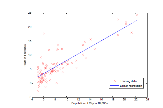
回归过程如图所示:
至此,我们通过梯度下降法解决了此问题,我们还可以通过之前所说的数学方法来解决,但是对于数据太大的情况(通常大于10000),我们就会通过梯度下降法来解决了
根据以上函数,我们进行线性回归:
最新文章
- BAT常用脚本汇总
- 移动web开发准备知识点
- C++的STL中vector内存分配方法的简单探索
- 原生Android动作
- 取得inputStream的长度
- 【解决】Microsoft Visual Studio 2012 打开2008下编译的silverlight3项目
- 3D视频的质量评价报告 (MSU出品)
- Keil MDK入门---从新建一个工程开始
- open live writer下载安装
- ORA-39002 ORA-39070 ORA-29283 ORA-06512 ORA-29283
- 关于ORACLE通过file_id与block_id定位数据库对象遇到的问题的一点思考
- Android图表库MPAndroidChart(十一)——多层级的堆叠条形图
- 阅读OReilly.Web.Scraping.with.Python.2015.6笔记---找出网页中所有的href
- 【Web安全】越权操作——横向越权与纵向越权
- 网站搜索引擎优化(SEO)的18条守则
- spring boot 定时备份数据库
- linux -- 进程的查看、进程id的获取、进程的杀死
- ZLYD团队第三周项目总结
- Mysql 优化与测试
- thinkphp htmlspecialchars_decode