[Pandas] 01 - A guy based on NumPy
主要搞明白NumPy “为什么快”?
一、学习资源
- Panda 中文
- 易百教程
- 远程登录Jupyter笔记本
- "第六章、矩阵和矢量计算" from《Python高性能编程》
- 系统级性能分析工具perf的介绍与使用
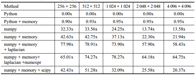
二、效率进化
NumPy 底层进行了不错的优化。
loops = 25000000

from math import *

# 策略1:对每一个元素依次进行计算
a = range(1, loops)

def f(x):

    return 3 * log(x) + cos(x) ** 2

%timeit r = [f(x) for x in a]
1 loop, best of 3: 14.4 s per loop
# 策略2:使用np

import numpy as np

a = np.arange(1, loops)

%timeit r = 3 * np.log(a) + np.cos(a) ** 2
10 loops, best of 3: 1.94 s per loop
# 策略3:numexpr方法,避免了数组在内存中复制

import numexpr as ne

ne.set_num_threads(1)

f = '3 * log(a) + cos(a) ** 2'
%timeit r = ne.evaluate(f)
10 loops, best of 3: 373 ms per loop
# 策略4:再并发四线程
ne.set_num_threads(4)  # 支持并发

%timeit r = ne.evaluate(f)
100 loops, best of 3: 195 ms per loop
三、高级知识点
(a) numexpr
NumPy 虽然通过底层高度优化过的计算库可以实现接近C的高效计算,但在计算复杂且计算量庞大的时候多少还是有些嫌慢。Numexpr 库是最近发现的一个非常简单易用的 Numpy性能提升工具。
Goto: NumExpr: Fast numerical expression evaluator for NumPy
(b) cupy利用gpu加速
先安装cuda驱动:[CUDA] 00 - GPU Driver Installation & Concurrency Programming
再安装CuPy驱动:CuPy Installation
(c) PyPy 与 CPython
需要了解:PyPy和CPython的不同点。
CPython的思路
def add(x, y):

    return x + y

if instance_has_method(x, '__add__') {

    return call(x, '__add__', y)   // x.__add__ 里面又有一大堆针对不同类型的 y 的判断

} else if isinstance_has_method(super_class(x), '__add__' {

    return call(super_class, '__add__', y)

} else if isinstance(x, str) and isinstance(y, str) {

    return concat_str(x, y)

} else if isinstance(x, float) and isinstance(y, float) {

    return add_float(x, y)

} else if isinstance(x, int) and isinstance(y, int) {

    return add_int(x, y)

} else ...
Just In Time 编译
为何加速了呢?PyPy 执行的时候,发现执行了一百遍 add 函数,发现你 TM 每次都只传两个整数进来,那我何苦每次还给你做这么多计算。于是当场生成了一个类似 C 的函数:
int add_int_int(int x, int y) {

  return x + y;

}
系统级性能剖析
一、原始实验
原始代码,作为之后的优化参照。
import numpy as np

import time

grid_size = (512,)

def laplacian(grid, out):

    np.copyto(out, grid)

    np.multiply(out, -2.0, out)

    np.add(out, np.roll(grid, +1), out)

    np.add(out, np.roll(grid, -1), out)

def evolve(grid, dt, out, D=1):

    laplacian(grid, out)

    np.multiply(out, D * dt, out)

    np.add(out, grid, out)


def run_experiment(num_iterations):

    scratch = np.zeros(grid_size)

    grid    = np.zeros(grid_size)

    block_low  = int(grid_size[0] * .4)

    block_high = int(grid_size[0] * .5)

    grid[block_low:block_high] = 0.005

    start = time.time()

    for i in range(num_iterations):

        evolve(grid, 0.1, scratch)

        grid, scratch = scratch, grid

    return time.time() - start


if __name__ == "__main__":

    run_experiment(500)
性能分析一:
$ sudo perf stat -e cycles,stalled-cycles-frontend,stalled-cycles-backend,instructions,cache-references,cache-misses,branches,branch-misses,task-clock,faults,minor-faults,cs,migrations -r 3 python diffusion_python_memory.py
 Performance counter stats for '/usr/local/anaconda3/bin/python3 diffusion_numpy_memory.py' ( runs):

               cycles                    #    3.605 GHz                      ( +-  2.30% )  (65.11%)

   <not supported>      stalled-cycles-frontend

   <not supported>      stalled-cycles-backend

               instructions              #    1.27  insn per cycle           ( +-  1.22% )  (82.56%)

                cache-references          #  231.400 M/sec                    ( +-  0.56% )  (82.71%)

                 cache-misses              #    8.797 % of all cache refs      ( +- 15.29% )  (83.90%)

               branches                  # 1011.101 M/sec                    ( +-  1.59% )  (83.90%)

                 branch-misses             #    2.99% of all branches          ( +-  0.49% )  (84.38%)

             99.34 msec task-clock                #    0.996 CPUs utilized            ( +-  4.31% )

                    faults                    #    0.050 M/sec                    ( +-  0.07% )

                    minor-faults              #    0.050 M/sec                    ( +-  0.07% )

                       cs                        #    0.007 K/sec                    ( +- 50.00% )

                       migrations                #    0.000 K/sec

           0.09976 +- 0.00448 seconds time elapsed  ( +-  4.49% )
二、利用内建优化代码
写在一起的好处是:短代码往往意味着高性能,因为容易利用内建优化机制。
def laplacian(grid):

    return np.roll(grid, +1) + np.roll(grid, -1) - 2 * grid


def evolve(grid, dt, D=1):

    return grid + dt * D * laplacian(grid)
性能分析二:cache-references非常大,但0.97指令减少才是重点。
 Performance counter stats for '/usr/local/anaconda3/bin/python3 diffusion_numpy.py' ( runs):

               cycles                    #    3.368 GHz                      ( +-  2.05% )  (63.87%)

   <not supported>      stalled-cycles-frontend

   <not supported>      stalled-cycles-backend

               instructions              #    1.28  insn per cycle           ( +-  0.41% )  (82.69%)

                cache-references          #  218.428 M/sec                    ( +-  0.44% )  (84.39%)

                 cache-misses              #   10.430 % of all cache refs      ( +-  4.03% )  (84.39%)

                branches                  #  962.634 M/sec                    ( +-  1.17% )  (84.39%)

                 branch-misses             #    2.99% of all branches          ( +-  0.24% )  (82.97%)

            102.48 msec task-clock                #    0.998 CPUs utilized            ( +-  2.02% )

                    faults                    #    0.049 M/sec                    ( +-  0.04% )

                    minor-faults              #    0.049 M/sec                    ( +-  0.04% )

                       cs                        #    0.007 K/sec                    ( +- 50.00% )

                       migrations                #    0.000 K/sec

           0.10270 +- 0.00209 seconds time elapsed  ( +-  2.04% )
三、降低内存分配、提高指令效率
找到 “正确的优化” 的点
我们使用 numpy降低了 CPU 负担,我们降低了解决问题所必要的内存分配次数。
事实上 evolve 函数有 93%的时间花费在 laplacian 函数中。
参见:[Optimized Python] 17 - Bottle-neck in performance
进一步优化
向操作系统进行请求所需的开销比简单填充缓存大很多。
填充一次缓存失效是一个在主板上优化过的硬件行为,而内存分配则需要跟另一个进程、内核打交道来完成。
(1)"+="运算符的使用减少了“不必要的变量内存分配”。
(2)roll_add替代过于全能的np.roll,以减少不必要的指令。
def roll_add(rollee, shift, out):

    if shift == :

        out[:] += rollee[:-]

        out[] += rollee[-]

    elif shift == -:

        out[:-] += rollee[:]

        out[-] += rollee[]

def laplacian(grid, out):

    np.copyto(out, grid)

    np.multiply(out, -2.0, out)

    roll_add(grid, +, out)

    roll_add(grid, -, out)

def evolve(grid, dt, out, D=1):

    laplacian(grid, out)

    np.multiply(out, D * dt, out)

    np.add(out, grid, out
性能分析三:减低了内存缺页,提高了指令效率。
 Performance counter stats for '/usr/local/anaconda3/bin/python3 diffusion_numpy_memory2.py' ( runs):

               cycles                    #    3.670 GHz                      ( +-  1.89% )  (62.67%)

   <not supported>      stalled-cycles-frontend

   <not supported>      stalled-cycles-backend

               instructions              #    1.28  insn per cycle           ( +-  0.19% )  (81.33%)

                cache-references          #  211.611 M/sec                    ( +-  2.65% )  (81.94%)

                 cache-misses              #   12.672 % of all cache refs      ( +-  6.84% )  (84.68%)

                branches                  # 1034.575 M/sec                    ( +-  0.68% )  (86.00%)

                 branch-misses             #    3.25% of all branches          ( +-  1.19% )  (84.71%)

             85.71 msec task-clock                #    0.997 CPUs utilized            ( +-  1.86% )

                    faults                    #    0.058 M/sec                    ( +-  0.10% )

                    minor-faults              #    0.058 M/sec                    ( +-  0.10% )

                       cs                        #    0.004 K/sec                    ( +-100.00% )

                       migrations                #    0.000 K/sec

           0.08596 +- 0.00163 seconds time elapsed  ( +-  1.89% )
四、整体处理表达式
numexpr 的一个重要特点是它考虑到了 CPU 缓存。它特地移动数据来让各级CPU 缓存能够拥有正确的数据让缓存失效最小化。
(a)当我们增加矩阵的大小时,我们会发现 numexpr 比原生 numpy 更好地利用了我们的缓存。而且,numexpr 利用了多核来进行计算并尝试填满每个核心的缓存。
(b)当矩阵较小时,管理多核的开销盖过了任何可能的性能提升。
import numexpr as ne

def evolve(grid, dt, out, D=):

    laplacian(grid, out)

    ne.evaluate("out*D*dt+grid", out=out)
性能分析四:减低了内存缺页,提高了指令效率。
 Performance counter stats for '/usr/local/anaconda3/bin/python3 diffusion_numpy_memory2_numexpr.py' ( runs):

               cycles                    #    3.888 GHz                      ( +-  1.01% )  (65.40%)

   <not supported>      stalled-cycles-frontend

   <not supported>      stalled-cycles-backend

               instructions              #    1.23  insn per cycle           ( +-  1.70% )  (82.72%)

                cache-references          #  232.372 M/sec                    ( +-  0.91% )  (82.89%)

                 cache-misses              #   10.513 % of all cache refs      ( +- 10.84% )  (83.77%)

               branches                  # 1032.639 M/sec                    ( +-  1.21% )  (84.97%)

                 branch-misses             #    3.21% of all branches          ( +-  0.61% )  (82.97%)

            100.18 msec task-clock                #    1.000 CPUs utilized            ( +-  5.75% )

                    faults                    #    0.086 M/sec                    ( +-  0.01% )

                    minor-faults              #    0.086 M/sec                    ( +-  0.01% )

                      cs                        #    0.123 K/sec                    ( +-  2.70% )

                       migrations                #    0.030 K/sec

           0.10018 +- 0.00582 seconds time elapsed  ( +-  5.81% )
五、利用现成的方案
直接使用scipy提供的接口。
from scipy.ndimage.filters import laplace

def laplacian(grid, out):

    laplace(grid, out, mode='wrap')
性能分析五:可能过于通用而没有明显提升。
 Performance counter stats for '/usr/local/anaconda3/bin/python3 diffusion_scipy.py' ( runs):

               cycles                    #    3.647 GHz                      ( +-  0.37% )  (63.49%)

   <not supported>      stalled-cycles-frontend

   <not supported>      stalled-cycles-backend

               instructions              #    1.28  insn per cycle           ( +-  1.10% )  (81.74%)

                cache-references          #  223.757 M/sec                    ( +-  0.37% )  (82.77%)

                 cache-misses              #    9.848 % of all cache refs      ( +-  1.46% )  (84.55%)

          96943942      branches                  # 1021.088 M/sec                    ( +-  0.80% )  (85.19%)

                 branch-misses             #    3.22% of all branches          ( +-  1.27% )  (84.00%)

             94.94 msec task-clock                #    0.997 CPUs utilized            ( +- 11.09% )

                    faults                    #    0.054 M/sec                    ( +-  0.10% )

                    minor-faults              #    0.054 M/sec                    ( +-  0.10% )

                       cs                        #    0.004 K/sec                    ( +-100.00% )

                       migrations                #    0.000 K/sec

            0.0952 +- 0.0106 seconds time elapsed  ( +- 11.14% )
六、总结
看来,scipy没有大的必要,“定制的” 优化比较靠谱。
NumPy Data Structures
使用原生 List 作为 Array
v = [0.5, 0.75, 1.0, 1.5, 2.0] # vector of numbers
m = [v, v, v]  # matrix of numbers

m
[[0.5, 0.75, 1.0, 1.5, 2.0],

 [0.5, 0.75, 1.0, 1.5, 2.0],

 [0.5, 0.75, 1.0, 1.5, 2.0]]
m[1]
[0.5, 0.75, 1.0, 1.5, 2.0]
m[1][0]
0.5
v1 = [0.5, 1.5]

v2 = [1, 2]

m = [v1, v2]

c = [m, m]  # cube of numbers

c
[[[0.5, 1.5], [1, 2]], [[0.5, 1.5], [1, 2]]]
c[1][1][0]
1
v = [0.5, 0.75, 1.0, 1.5, 2.0]

m = [v, v, v]

m
[[0.5, 0.75, 1.0, 1.5, 2.0],

 [0.5, 0.75, 1.0, 1.5, 2.0],

 [0.5, 0.75, 1.0, 1.5, 2.0]]
v[0] = 'Python'

m
[['Python', 0.75, 1.0, 1.5, 2.0],

 ['Python', 0.75, 1.0, 1.5, 2.0],

 ['Python', 0.75, 1.0, 1.5, 2.0]]
from copy import deepcopy

v = [0.5, 0.75, 1.0, 1.5, 2.0]

m = 3 * [deepcopy(v), ]

m
[[0.5, 0.75, 1.0, 1.5, 2.0],

 [0.5, 0.75, 1.0, 1.5, 2.0],

 [0.5, 0.75, 1.0, 1.5, 2.0]]
v[0] = 'Python'

m
[[0.5, 0.75, 1.0, 1.5, 2.0],

 [0.5, 0.75, 1.0, 1.5, 2.0],

 [0.5, 0.75, 1.0, 1.5, 2.0]]
使用 NumPy Arrays
import numpy as np
a = np.array([0, 0.5, 1.0, 1.5, 2.0])

type(a)
numpy.ndarray
a[:2] # indexing as with list objects in 1 dimension
array([ 0. , 0.5])
a.sum() # sum of all elements
5.0
a.std() # standard deviation
0.70710678118654757
a.cumsum() # running cumulative sum
array([ 0. , 0.5, 1.5, 3. , 5. ])
a * 2
array([ 0., 1., 2., 3., 4.])
a ** 2
array([ 0. , 0.25, 1. , 2.25, 4. ])
np.sqrt(a)
array([ 0. , 0.70710678, 1. , 1.22474487, 1.41421356])
b = np.array([a, a * 2])

b
array([[ 0. ,  0.5,  1. ,  1.5,  2. ],

       [ 0. ,  1. ,  2. ,  3. ,  4. ]])
b[0] # first row
array([ 0. , 0.5, 1. , 1.5, 2. ])
b[0, 2] # third element of first row
1.0
b.sum()
15.0
b.sum(axis=0)

  # sum along axis 0, i.e. column-wise sum
array([ 0. , 1.5, 3. , 4.5, 6. ])
b.sum(axis=1)

  # sum along axis 1, i.e. row-wise sum
array([ 5., 10.])
c = np.zeros((2, 3, 4), dtype='i', order='C')  # also: np.ones()

c
array([[[0, 0, 0, 0],

        [0, 0, 0, 0],

        [0, 0, 0, 0]],

       [[0, 0, 0, 0],

        [0, 0, 0, 0],

        [0, 0, 0, 0]]], dtype=int32)
d = np.ones_like(c, dtype='f16', order='C')  # also: np.zeros_like()

d
array([[[ 1.0,  1.0,  1.0,  1.0],

        [ 1.0,  1.0,  1.0,  1.0],

        [ 1.0,  1.0,  1.0,  1.0]],

       [[ 1.0,  1.0,  1.0,  1.0],

        [ 1.0,  1.0,  1.0,  1.0],

        [ 1.0,  1.0,  1.0,  1.0]]], dtype=float128)
import random

I = 5000
%time mat = [[random.gauss(0, 1) for j in range(I)] for i in range(I)]

  # a nested list comprehension
CPU times: user 21.3 s, sys: 238 ms, total: 21.5 s

Wall time: 21.5 s
%time mat = np.random.standard_normal((I, I))
CPU times: user 1.36 s, sys: 55.9 ms, total: 1.42 s

Wall time: 1.42 s
%time mat.sum()
CPU times: user 15.2 ms, sys: 0 ns, total: 15.2 ms

Wall time: 14.1 ms
1137.43504265149
自定义 Arrays
dt = np.dtype([('Name', 'S10'), ('Age', 'i4'),

               ('Height', 'f'), ('Children/Pets', 'i4', 2)])  # 类似与数据库的表,定义列的属性;每列数据的类型是要确保一致的

s = np.array([('Smith', 45, 1.83, (0, 1)),

              ('Jones', 53, 1.72, (2, 2))], dtype=dt)

s
array([(b'Smith', 45,  1.83000004, [0, 1]),

       (b'Jones', 53,  1.72000003, [2, 2])],

      dtype=[('Name', 'S10'), ('Age', '<i4'), ('Height', '<f4'), ('Children/Pets', '<i4', (2,))])
s['Name']
array([b'Smith', b'Jones'],

      dtype='|S10')
s['Height'].mean()
1.7750001
s[1]['Age']
53
Vectorization of Code
Basic Vectorization 向量化
r = np.random.standard_normal((4, 3))

s = np.random.standard_normal((4, 3))
r + s
array([[  1.33110811e+00,   1.26931718e+00,   4.43935711e-01],

       [ -1.06905167e+00,   1.38422425e+00,  -1.99126769e+00],

       [  3.24832612e-01,  -6.63041986e-01,  -1.11329038e+00],

       [  6.53171734e-01,  -1.69497518e-05,   3.48108030e-01]])
2 * r + 3
array([[ 6.23826763,  3.4056893 ,  4.93537977],

       [ 3.41201018,  3.18058875,  0.07823276],

       [ 5.21407609,  2.93499984,  2.62703963],

       [ 6.23041052,  6.13968592,  2.783421  ]])
s = np.random.standard_normal(3)

r + s
array([[ 1.43696477, -0.89451367, -0.07713104],

       [ 0.02383604, -1.00706394, -2.50570454],

       [ 0.924869  , -1.12985839, -1.23130111],

       [ 1.43303621,  0.47248465, -1.15311042]])
# causes intentional error

# s = np.random.standard_normal(4)

# r + s
# r.transpose() + s
np.shape(r.T)
(3, 4)
def f(x):

    return 3 * x + 5
f(0.5) # float object
6.5
f(r) # NumPy array
array([[ 9.85740144,  5.60853394,  7.90306966],

       [ 5.61801527,  5.27088312,  0.61734914],

       [ 8.32111413,  4.90249976,  4.44055944],

       [ 9.84561578,  9.70952889,  4.6751315 ]])
# causes intentional error

# import math

# math.sin(r)
np.sin(r) # array as input
array([[ 0.99883197,  0.20145647,  0.82357761],

       [ 0.2045511 ,  0.09017173, -0.99396568],

       [ 0.89437769, -0.03249436, -0.18540126],

       [ 0.99901409,  0.99999955, -0.10807798]])
np.sin(np.pi) # float as input
1.2246467991473532e-16
结构组织方式
x = np.random.standard_normal((5, 10000000))

y = 2 * x + 3  # linear equation y = a * x + b

C = np.array((x, y), order='C')          # 按行统计快些

F = np.array((x, y), order='F')          # 按列统计快些

x = 0.0; y = 0.0  # memory clean-up
C[:2].round(2) # 四舍五入
array([[[ 1.51,  0.67, -0.96, ..., -0.71, -1.55,  2.49],

        [ 0.65, -0.15,  0.02, ...,  0.49, -0.26,  1.37],

        [-0.07,  0.74, -2.31, ..., -0.51,  0.52,  0.49],

        [ 0.52, -0.43, -0.18, ..., -0.06,  0.58,  1.46],

        [-0.32,  0.59, -0.75, ..., -0.03,  0.23, -0.75]],

       [[ 6.01,  4.35,  1.07, ...,  1.58, -0.11,  7.97],

        [ 4.3 ,  2.71,  3.04, ...,  3.99,  2.48,  5.75],

        [ 2.86,  4.48, -1.62, ...,  1.97,  4.04,  3.97],

        [ 4.03,  2.14,  2.63, ...,  2.88,  4.16,  5.92],

        [ 2.36,  4.19,  1.51, ...,  2.94,  3.46,  1.5 ]]])
%timeit C.sum()
10 loops, best of 3: 45.2 ms per loop
%timeit F.sum()
10 loops, best of 3: 48.2 ms per loop
%timeit C[0].sum(axis=0)
10 loops, best of 3: 66.4 ms per loop
%timeit C[0].sum(axis=1)
10 loops, best of 3: 22.8 ms per loop
%timeit F.sum(axis=0)
1 loop, best of 3: 712 ms per loop
%timeit F.sum(axis=1)
1 loop, best of 3: 1.64 s per loop
F = 0.0; C = 0.0 # memory clean-up
最新文章
- windows下制作linux U盘启动盘或者安装优盘(转)
- question2answer论坛框架分析及web开发思考
- MySQL日志恢复误删记录
- MySQL auto-extending data file
- @Valid springMVC bean校验不起作用
- iOS开发--TableView详细解释
- 读 Runtime 源码:对象与引用计数
- 轻量级表格插件Bootstrap Table。拥有强大的支持固定表头、单/复选、排序、分页、搜索及自定义表头等功能。
- .net邮件发送帮助类
- python操作Excel-写/改/读
- ajax-page局部刷新分页实例
- python 常用模块之random,os,sys 模块
- [POJ 3984] 迷宫问题(BFS最短路径的记录和打印问题)
- webpack+vue-cli中代理配置(proxyTable)
- php iframe 上传文件
- 三种数据库访问——Spring JDBC
- 百度地图地址解析(百度Geocoding API)
- javascript关闭网页的几种方法
- JDBC及DBUtils
- jdbc关闭连接顺序