《DSP using MATLAB》Problem 8.42
2024-08-29 19:05:56
代码:
%% ------------------------------------------------------------------------

%%            Output Info about this m-file

fprintf('\n***********************************************************\n');

fprintf('        <DSP using MATLAB> Problem 8.42 \n\n');

banner();

%% ------------------------------------------------------------------------

% Digital Filter Specifications:   Elliptic bandstop

wsbs = [0.40*pi 0.48*pi];             % digital stopband freq in rad

wpbs = [0.25*pi 0.75*pi];             % digital passband freq in rad

Rp = 1.0    % passband ripple in dB

As = 80      % stopband attenuation in dB

Ripple = 10 ^ (-Rp/20)           % passband ripple in absolute

Attn = 10 ^ (-As/20)             % stopband attenuation in absolute

% Calculation of Elliptic filter parameters:

[N, wn] = ellipord(wpbs/pi, wsbs/pi, Rp, As);

fprintf('\n  ********* Elliptic Digital Bandstop Filter Order is = %3.0f \n', 2*N)

% Digital Elliptic bandstop Filter Design:

[bbs, abs] = ellip(N, Rp, As, wn, 'stop');

[C, B, A] = dir2cas(bbs, abs)

% Calculation of Frequency Response:

[dbbs, magbs, phabs, grdbs, wwbs] = freqz_m(bbs, abs);

% ---------------------------------------------------------------

%    find Actual Passband Ripple and Min Stopband attenuation

% ---------------------------------------------------------------

delta_w = 2*pi/1000;

Rp_bs = -(min(dbbs(1:1:ceil(wpbs(1)/delta_w+1))));                           % Actual Passband Ripple

fprintf('\nActual Passband Ripple is %.4f dB.\n', Rp_bs);

As_bs = -round(max(dbbs(ceil(wsbs(1)/delta_w)+1:1:ceil(wsbs(2)/delta_w)+1)));   % Min Stopband attenuation

fprintf('\nMin Stopband attenuation is %.4f dB.\n\n', As_bs);

%% -----------------------------------------------------------------

%%                             Plot

%% -----------------------------------------------------------------

figure('NumberTitle', 'off', 'Name', 'Problem 8.42 Elliptic bs by ellip function')

set(gcf,'Color','white');

M = 1;                          % Omega max

subplot(2,2,1); plot(wwbs/pi, magbs); axis([0, M, 0, 1.2]); grid on;

xlabel('Digital frequency in \pi units'); ylabel('|H|'); title('Magnitude Response');

set(gca, 'XTickMode', 'manual', 'XTick', [0, 0.25, 0.40, 0.48, 0.75, M]);

set(gca, 'YTickMode', 'manual', 'YTick', [0, 0.01, 0.8913, 1]);

subplot(2,2,2); plot(wwbs/pi, dbbs); axis([0, M, -120, 2]); grid on;

xlabel('Digital frequency in \pi units'); ylabel('Decibels'); title('Magnitude in dB');

set(gca, 'XTickMode', 'manual', 'XTick', [0, 0.25, 0.40, 0.48, 0.75, M]);

set(gca, 'YTickMode', 'manual', 'YTick', [ -80, -40, 0]);

set(gca,'YTickLabelMode','manual','YTickLabel',['80'; '40';' 0']);

subplot(2,2,3); plot(wwbs/pi, phabs/pi); axis([0, M, -1.1, 1.1]); grid on;

xlabel('Digital frequency in \pi nuits'); ylabel('radians in \pi units'); title('Phase Response');

set(gca, 'XTickMode', 'manual', 'XTick', [0, 0.25, 0.40, 0.48, 0.75, M]);

set(gca, 'YTickMode', 'manual', 'YTick', [-1:0.5:1]);

subplot(2,2,4); plot(wwbs/pi, grdbs); axis([0, M, 0, 50]); grid on;

xlabel('Digital frequency in \pi units'); ylabel('Samples'); title('Group Delay');

set(gca, 'XTickMode', 'manual', 'XTick', [0, 0.25, 0.40, 0.48, 0.75, M]);

set(gca, 'YTickMode', 'manual', 'YTick', [0:20:50]);

% ------------------------------------------------------------

%                 PART 2

% ------------------------------------------------------------

% Discrete time signal

Ts = 1;                              % sample intevals

n1_start = 0; n1_end = 200;

      n1 = [n1_start:n1_end];        % [0:200]

xn1 = sin(0.44*pi*n1);               % digital signal

% ----------------------------

%       DTFT of xn1

% ----------------------------

M = 500;

[X1, w] = dtft1(xn1, n1, M);

%magX1 = abs(X1);

angX1  = angle(X1);  realX1  = real(X1);  imagX1  = imag(X1);

magX1 = sqrt(realX1.^2 + imagX1.^2);

%% --------------------------------------------------------------------

%%              START X(w)'s  mag ang real imag

%% --------------------------------------------------------------------

figure('NumberTitle', 'off', 'Name', 'Problem 8.42 X1 DTFT');

set(gcf,'Color','white');

subplot(2,1,1); plot(w/pi,magX1); grid on;  %axis([-1,1,0,1.05]);

title('Magnitude Response');

xlabel('digital frequency in \pi units'); ylabel('Magnitude  |H|');

set(gca, 'XTickMode', 'manual', 'XTick', [0, 0.2, 0.44, 0.6, 0.8, 1.0, 1.2, 1.4, 1.56, 1.8, 2]);

subplot(2,1,2); plot(w/pi, angX1/pi); grid on;  %axis([-1,1,-1.05,1.05]);

title('Phase Response');

xlabel('digital frequency in \pi units'); ylabel('Radians/\pi');

figure('NumberTitle', 'off', 'Name', 'Problem 8.42 X1 DTFT');

set(gcf,'Color','white');

subplot(2,1,1); plot(w/pi, realX1); grid on;

title('Real Part');

xlabel('digital frequency in \pi units'); ylabel('Real');

set(gca, 'XTickMode', 'manual', 'XTick', [0, 0.2, 0.44, 0.6, 0.8, 1.0, 1.2, 1.4, 1.56, 1.8, 2]);

subplot(2,1,2); plot(w/pi, imagX1); grid on;

title('Imaginary Part');

xlabel('digital frequency in \pi units'); ylabel('Imaginary');

%% -------------------------------------------------------------------

%%             END X's  mag ang real imag

%% -------------------------------------------------------------------

% ------------------------------------------------------------

%                 PART 3

% ------------------------------------------------------------

yn1 = filter(bbs, abs, xn1);

n2 = n1;

% ----------------------------

%       DTFT of yn1

% ----------------------------

M = 500;

[Y1, w] = dtft1(yn1, n2, M);

%magY1  = abs(Y1);

angY1  = angle(Y1);  realY1  = real(Y1);  imagY1  = imag(Y1);

magY1 = sqrt(realY1.^2 + imagY1.^2);

%% --------------------------------------------------------------------

%%              START Y1(w)'s  mag ang real imag

%% --------------------------------------------------------------------

figure('NumberTitle', 'off', 'Name', 'Problem 8.42 Y1 DTFT');

set(gcf,'Color','white');

subplot(2,1,1); plot(w/pi,magY1); grid on;  %axis([-1,1,0,1.05]);

title('Magnitude Response');

xlabel('digital frequency in \pi units'); ylabel('Magnitude  |H|');

subplot(2,1,2); plot(w/pi, angY1/pi); grid on;  %axis([-1,1,-1.05,1.05]);

title('Phase Response');

xlabel('digital frequency in \pi units'); ylabel('Radians/\pi');

figure('NumberTitle', 'off', 'Name', 'Problem 8.42 Y1 DTFT');

set(gcf,'Color','white');

subplot(2,1,1); plot(w/pi, realY1); grid on;

title('Real Part');

xlabel('digital frequency in \pi units'); ylabel('Real');

subplot(2,1,2); plot(w/pi, imagY1); grid on;

title('Imaginary Part');

xlabel('digital frequency in \pi units'); ylabel('Imaginary');

%% -------------------------------------------------------------------

%%             END Y1's  mag ang real imag

%% -------------------------------------------------------------------

figure('NumberTitle', 'off', 'Name', 'Problem 8.42 x(n) and y(n)')

set(gcf,'Color','white');

subplot(2,1,1); stem(n1, xn1);

xlabel('n'); ylabel('x(n)');

title('xn sequence');  grid on;

subplot(2,1,2); stem(n1, yn1);

xlabel('n'); ylabel('y(n)');

title('yn sequence');  grid on;
运行结果:
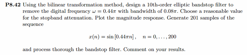
我自己假设通带1dB,阻带衰减80dB。
在此基础上设计指标,绝对单位,
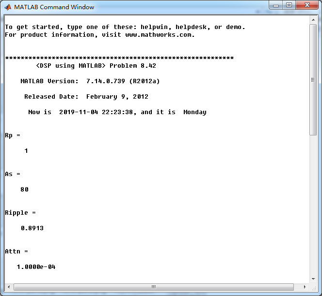
ellip函数(MATLAB工具箱函数)得到Elliptic带阻滤波器,阶数为10,系统函数串联形式系数如下图。
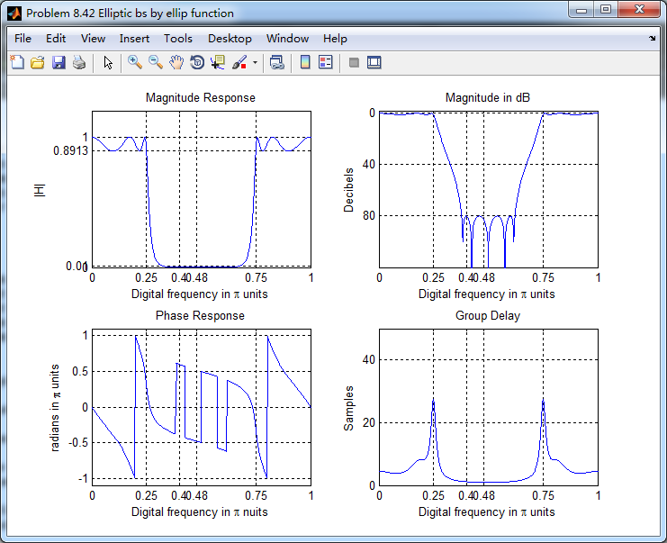
Elliptic带阻滤波器,幅度谱、相位谱和群延迟响应
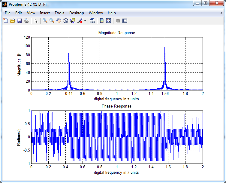
输入离散时间信号x(n)的谱如下,可看出,频率分量0.44π
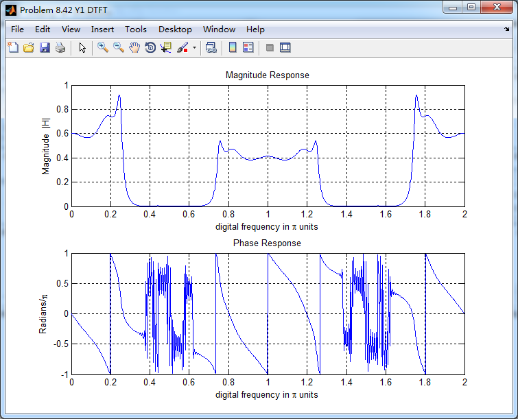
通过带阻滤波器后,得到的输出y(n)的谱,好像变乱了,o(╥﹏╥)o
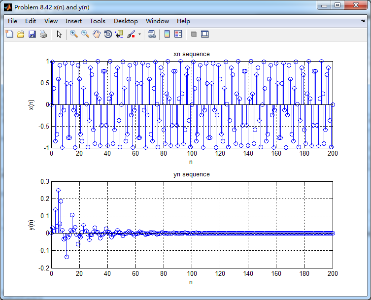
输入和输出的离散时间序列如下图
最新文章
- Visual Studio 2010的MSDN帮助文档离线使用
- 取消IE默认下载工具为迅雷
- jq数组,得到遍历生成的id后面的id
- 为什么需要DTO(数据传输对象)
- debian清除无用的库文件(清理系统,洁癖专用)
- 1874 素数和最大 - Wikioi
- mysqldump原理4
- KALI ssh无法登陆的解决办法
- angularjs中的绑定策略“@”,“=”,“&”实例
- maven+springmvc+easyui+fastjson+pagehelper
- 集装箱学习(两):动手模拟AOP
- js 控制随机数生成概率
- phpStrom映射代码
- Matlab调用Java类
- Pycharm 的设置--参数设置(运行.py文件带参数,例如argument)
- 编程语言,执行python程序,变量(命名规范)
- flask重要点
- 关于TP5.0搜索后分页
- ajax+ashx:实现文件的批量导出
- linux(centos 7)下安装elasticsearch 5 的 IK 分词器