机器学习作业(一)线性回归——Matlab实现
2024-09-06 20:31:15
题目太长啦!文档下载【传送门】
第1题
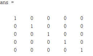
简述:设计一个5*5的单位矩阵。
function A = warmUpExercise()

A = [];

A = eye(5);

end
运行结果:
第2题
简述:实现单变量线性回归。
第1步:加载数据文件;
data = load('ex1data1.txt');

X = data(:, 1); y = data(:, 2);

m = length(y); % number of training examples

% Plot Data

% Note: You have to complete the code in plotData.m

plotData(X, y);
第2步:plotData函数实现训练样本的可视化;
function plotData(x, y)

figure;

plot(x,y,'rx','MarkerSize',10);

ylabel('Profit in $10,000s');

xlabel('Population of City in 10,000s');

end
第3步:使用梯度下降函数计算局部最优解,并显示线性回归;
X = [ones(m, 1), data(:,1)]; % Add a column of ones to x

theta = zeros(2, 1); % initialize fitting parameters

% Some gradient descent settings

iterations = 1500;

alpha = 0.01;

% run gradient descent

theta = gradientDescent(X, y, theta, alpha, iterations);

% print theta to screen

fprintf('Theta found by gradient descent:\n');

fprintf('%f\n', theta);

% Plot the linear fit

hold on; % keep previous plot visible

plot(X(:,2), X*theta, '-')

legend('Training data', 'Linear regression')

hold off % don't overlay any more plots on this figure
第4步:实现梯度下降gradientDescent函数;
function [theta, J_history] = gradientDescent(X, y, theta, alpha, num_iters)

% Initialize some useful values

m = length(y); % number of training examples

J_history = zeros(num_iters, 1);

for iter = 1:num_iters

    theta = theta - alpha/length(y)*(X'*(X*theta-y));

    % Save the cost J in every iteration

    J_history(iter) = computeCost(X, y, theta);

end

end
第5步:实现代价计算computeCost函数;
function J = computeCost(X, y, theta)

m = length(y); % number of training examples

J = 1/(2*m)*sum((X*theta-y).^2);

end
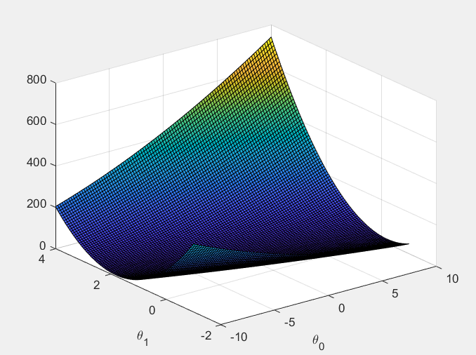
第6步:实现三维图、轮廓图的显示。
% Grid over which we will calculate J

theta0_vals = linspace(-10, 10, 100);

theta1_vals = linspace(-1, 4, 100);

% initialize J_vals to a matrix of 0's

J_vals = zeros(length(theta0_vals), length(theta1_vals));

% Fill out J_vals

for i = 1:length(theta0_vals)

    for j = 1:length(theta1_vals)

	  t = [theta0_vals(i); theta1_vals(j)];

	  J_vals(i,j) = computeCost(X, y, t);

    end

end

% Because of the way meshgrids work in the surf command, we need to

% transpose J_vals before calling surf, or else the axes will be flipped

J_vals = J_vals';

% Surface plot

figure;

surf(theta0_vals, theta1_vals, J_vals);

xlabel('\theta_0'); ylabel('\theta_1');

% Contour plot

figure;

% Plot J_vals as 15 contours spaced logarithmically between 0.01 and 100

contour(theta0_vals, theta1_vals, J_vals, logspace(-2, 3, 20))

xlabel('\theta_0'); ylabel('\theta_1');

hold on;

plot(theta(1), theta(2), 'rx', 'MarkerSize', 10, 'LineWidth', 2);
运行结果:


第3题
简述:实现多元线性回归。
第1步:加载数据文件;
data = load('ex1data2.txt');

X = data(:, 1:2);

y = data(:, 3);

m = length(y);

[X mu sigma] = featureNormalize(X);

% Add intercept term to X

X = [ones(m, 1) X];
第2步:均值归一化featureNormalize函数实现;
function [X_norm, mu, sigma] = featureNormalize(X)

X_norm = X;

mu = zeros(1, size(X, 2));

sigma = zeros(1, size(X, 2));

mu = mean(X,1);

sigma = std(X,0,1);

X_norm = (X_norm-mu)./sigma;

end
第3步:使用梯度下降函数计算局部最优解,并显示线性回归;
% Choose some alpha value

alpha = 0.05;

num_iters = 100;

% Init Theta and Run Gradient Descent

theta = zeros(3, 1);

[theta, J_history] = gradientDescentMulti(X, y, theta, alpha, num_iters);

% Plot the convergence graph

figure;

plot(1:numel(J_history), J_history, '-b', 'LineWidth', 2);

xlabel('Number of iterations');

ylabel('Cost J');
第4步:实现梯度下降gradientDescentMulti函数;
function [theta, J_history] = gradientDescentMulti(X, y, theta, alpha, num_iters)

m = length(y); % number of training examples

J_history = zeros(num_iters, 1);

for iter = 1:num_iters

    theta = theta - alpha/m*(X'*(X*theta-y));

    % Save the cost J in every iteration

    J_history(iter) = computeCostMulti(X, y, theta);

end

end
第5步:实现代价计算computeCostMulti函数;
function J = computeCostMulti(X, y, theta)

m = length(y); % number of training examples

J = 1/(2*m)*sum((X*theta-y).^2);%J=(X*theta-y)'*(X*theta-y)/(2*m);

end
运行结果:

第6步:使用上述结果对“the price of a 1650 sq-ft, 3 br house”进行预测;
X1 = [1,1650,3];

X1(2:3) = (X1(2:3)-mu)./sigma;

price = X1*theta;
预测结果:

第7步:使用正规方程法求解;
%%Load Data

data = csvread('ex1data2.txt');

X = data(:, 1:2);

y = data(:, 3);

m = length(y);

% Add intercept term to X

X = [ones(m, 1) X];

% Calculate the parameters from the normal equation

theta = normalEqn(X, y);
第8步:实现normalEqn函数;
function [theta] = normalEqn(X, y)

theta = zeros(size(X, 2), 1);

theta = (X'*X)^(-1)*X'*y;

end
第9步:使用上述结果对“the price of a 1650 sq-ft, 3 br house”再次进行预测;
price = [1,1650,3]*theta;
预测结果:(与梯度下降法结果很接近)

最新文章
- Linux 下 git连接github的使用
- iOS中关于.pch的新建与配置问题
- 【django】request
- Oracle 10g设置IP访问限制
- 黑盒测试用例设计方法&理论结合实际 -> 判定表驱动法
- JavaScript之面向对象学习二(原型属性对象与in操作符)获取对象中所有属性的方法
- asm 盘头损失,破坏
- wpf xmal基础
- CentOS6.4安装go环境
- setTimeout和setInterval不容易注意到的一些细节
- tensorflow 自定义损失函数示例
- vim 当前用户显示行号
- TypeScript入门(一)
- MySQL--BNL/ICP/MRR/BKA
- vba报表制作
- 01List.ashx(班级列表动态页面)
- eclipse 大括号 改为C语言风格
- es 之 Symbol
- Frosh Week
- bzoj 1115: [POI2009]石子游戏Kam -- 博弈论