改善深层神经网络-week3编程题(Tensorflow 实现手势识别 )
TensorFlow Tutorial
- Initialize variables
- Start your own session
- Train algorithms
- Implement a Neural Network
1. Exploring the Tensorflow Library
To start, you will import the library:
import math

import numpy as np

import h5py

import matplotlib.pyplot as plt

import tensorflow as tf

from tensorflow.python.framework import ops

from tf_utils import load_dataset, random_mini_batches, convert_to_one_hot, predict

%matplotlib inline

np.random.seed(1)
Now that you have imported the library, we will walk you through its different applications. You will start with an example, where we compute for you the loss of one training example.
\]
y_hat = tf.constant(36, name='y_hat')            # Define y_hat constant. Set to 36.

y = tf.constant(39, name='y')                    # Define y. Set to 39

loss = tf.Variable((y - y_hat)**2, name='loss')  # Create a variable for the loss

init = tf.global_variables_initializer()         # When init is run later (session.run(init)),

                                                 # the loss variable will be initialized and ready to be computed

with tf.Session() as session:                    # Create a session and print the output

    session.run(init)                            # Initializes the variables

    print(session.run(loss))                     # Prints the loss
Writing and running programs in TensorFlow has the following steps:
- Create Tensors (variables) that are not yet executed/evaluated.
- Write operations between those Tensors.
- Initialize your Tensors.
- Create a Session.
- Run the Session. This will run the operations you'd written above.
1.1 - Linear function
Lets start this programming exercise by computing the following equation: \(Y = WX + b\), where \(W\) and \(X\) are random matrices and b is a random vector.
Exercise: Compute \(WX + b\) where \(W, X\), and \(b\) are drawn from a random normal distribution. W is of shape (4, 3), X is (3,1) and b is (4,1). As an example, here is how you would define a constant X that has shape (3,1):
X = tf.constant(np.random.randn(3,1), name = "X")
You might find the following functions helpful:
- tf.matmul(..., ...) to do a matrix multiplication
- tf.add(..., ...) to do an addition
- np.random.randn(...) to initialize randomly
# GRADED FUNCTION: linear_function

def linear_function():

    """

    Implements a linear function:

            Initializes W to be a random tensor of shape (4,3)

            Initializes X to be a random tensor of shape (3,1)

            Initializes b to be a random tensor of shape (4,1)

    Returns:

    result -- runs the session for Y = WX + b

    """

    np.random.seed(1)

    ### START CODE HERE ### (4 lines of code)

    W = tf.constant(np.random.randn(4, 3), name='W')

    X = tf.constant(np.random.randn(3, 1), name='X')

    b = tf.constant(np.random.randn(4, 1), name='b')

    Y = tf.add(tf.matmul(W, X), b)

    ### END CODE HERE ###

    # Create the session using tf.Session() and run it with sess.run(...) on the variable you want to calculate

    ### START CODE HERE ###

    sess = tf.Session()

    result = sess.run(Y)

    ### END CODE HERE ###

    # close the session

    sess.close()

    return result
1.2 - Computing the sigmoid
Great! You just implemented a linear function. Tensorflow offers a variety of commonly used neural network functions like tf.sigmoid and tf.softmax. For this exercise lets compute the sigmoid function of an input.
You will do this exercise using a placeholder variable x. When running the session, you should use the feed dictionary to pass in the input z. In this exercise, you will have to (i) create a placeholder x, (ii) define the operations needed to compute the sigmoid using tf.sigmoid, and then (iii) run the session.
** Exercise **: Implement the sigmoid function below. You should use the following:
tf.placeholder(tf.float32, name = "...")tf.sigmoid(...)sess.run(..., feed_dict = {x: z})
Note that there are two typical ways to create and use sessions in tensorflow:
Method 1:
sess = tf.Session()

# Run the variables initialization (if needed), run the operations

result = sess.run(..., feed_dict = {...})

sess.close() # Close the session
Method 2:
with tf.Session() as sess:

    # run the variables initialization (if needed), run the operations

    result = sess.run(..., feed_dict = {...})

    # This takes care of closing the session for you :)
print ("sigmoid(0) = " + str(sigmoid(0)))

print ("sigmoid(12) = " + str(sigmoid(12)))
输出:
sigmoid(0) = 0.5
sigmoid(12) = 0.9999942
**To summarize, you how know how to**:
1. Create placeholders
2. Specify the computation graph corresponding to operations you want to compute
3. Create the session
4. Run the session, using a feed dictionary if necessary to specify placeholder variables' values.
1.3 - Computing the Cost
You can also use a built-in function to compute the cost of your neural network. So instead of needing to write code to compute this as a function of \(a^{[2](i)}\) and \(y^{(i)}\) for i=1...m:
\]
you can do it in one line of code in tensorflow!
Exercise: Implement the cross entropy loss. The function you will use is:
tf.nn.sigmoid_cross_entropy_with_logits(logits = ..., labels = ...)
Your code should input z, compute the sigmoid (to get a) and then compute the cross entropy cost \(J\). All this can be done using one call to tf.nn.sigmoid_cross_entropy_with_logits, which computes
\]
# GRADED FUNCTION: cost

def cost(logits, labels):

    """

    Computes the cost using the sigmoid cross entropy


    Arguments:

    logits -- vector containing z, output of the last linear unit (before the final sigmoid activation)

    labels -- vector of labels y (1 or 0)

    Note: What we've been calling "z" and "y" in this class are respectively called "logits" and "labels"

    in the TensorFlow documentation. So logits will feed into z, and labels into y.


    Returns:

    cost -- runs the session of the cost (formula (2))

    """

    ### START CODE HERE ###

    z = tf.placeholder(tf.float32, name='z')

    y = tf.placeholder(tf.float32, name='y')

    # Use the loss function (approx. 1 line)

    cost = tf.nn.sigmoid_cross_entropy_with_logits(logits=z, labels=y)

    # Create a session (approx. 1 line). See method 1 above.

    sess = tf.Session()

    # Run the session (approx. 1 line).

    cost = sess.run(cost, feed_dict={z: logits, y:labels})

    # Close the session (approx. 1 line). See method 1 above.

    sess.close()

    ### END CODE HERE ###

    return cost
logits = sigmoid(np.array([0.2,0.4,0.7,0.9]))

cost = cost(logits, np.array([0,0,1,1]))

print ("cost = " + str(cost))
cost = [ 1.00538719 1.03664088 0.41385433 0.39956614]
1.4 - Using One Hot encodings
Many times in deep learning you will have a y vector with numbers ranging from 0 to C-1, where C is the number of classes. If C is for example 4, then you might have the following y vector which you will need to convert as follows:

This is called a "one hot" encoding, because in the converted representation exactly one element of each column is "hot" (meaning set to 1). To do this conversion in numpy, you might have to write a few lines of code. In tensorflow, you can use one line of code:
- tf.one_hot(labels, depth, axis)
Exercise: Implement the function below to take one vector of labels and the total number of classes \(C\), and return the one hot encoding. Use tf.one_hot() to do this.
# GRADED FUNCTION: one_hot_matrix

def one_hot_matrix(labels, C):

    """

    Creates a matrix where the i-th row corresponds to the ith class number and the jth column

                     corresponds to the jth training example. So if example j had a label i. Then entry (i,j)

                     will be 1.

    Arguments:

    labels -- vector containing the labels

    C -- number of classes, the depth of the one hot dimension

    Returns:

    one_hot -- one hot matrix

    """

    ### START CODE HERE ###

    # Create a tf.constant equal to C (depth), name it 'C'. (approx. 1 line)

    C = tf.constant(C, name='C')

    # Use tf.one_hot, be careful with the axis (approx. 1 line)

    one_hot_matrix = tf.one_hot(indices=labels, depth=C, axis=0)

    # Create the session (approx. 1 line)

    sess = tf.Session()

    # Run the session (approx. 1 line)

    one_hot = sess.run(one_hot_matrix)

    # Close the session (approx. 1 line). See method 1 above.

    sess.close()

    ### END CODE HERE ###

    return one_hot
输出:
labels = np.array([1,2,3,0,2,1])

one_hot = one_hot_matrix(labels, C = 4)

print ("one_hot = " + str(one_hot))
1.5 - Initialize with zeros and ones
Now you will learn how to initialize a vector of zeros and ones. The function you will be calling is tf.ones(). To initialize with zeros you could use tf.zeros() instead. These functions take in a shape and return an array of dimension shape full of zeros and ones respectively.
Exercise: Implement the function below to take in a shape and to return an array (of the shape's dimension of ones).
- tf.ones(shape)
# GRADED FUNCTION: ones

def ones(shape):

    """

    Creates an array of ones of dimension shape

    Arguments:

    shape -- shape of the array you want to create

    Returns:

    ones -- array containing only ones

    """

    ### START CODE HERE ###

    # Create "ones" tensor using tf.ones(...). (approx. 1 line)

    ones = tf.ones(shape)

    # Create the session (approx. 1 line)

    sess = tf.Session()

    # Run the session to compute 'ones' (approx. 1 line)

    ones = sess.run(ones)

    # Close the session (approx. 1 line). See method 1 above.

    sess.close()

    ### END CODE HERE ###

    return ones
测试:
print ("ones = " + str(ones([3])))
2 - Building your first neural network in tensorflow
In this part of the assignment you will build a neural network using tensorflow. Remember that there are two parts to implement a tensorflow model:
- Create the computation graph
- Run the graph
Let's delve into the problem you'd like to solve!
2.0 - Problem statement: SIGNS Dataset
手势数字识别
- Training set: 1080 pictures (64 by 64 pixels) of signs representing numbers from 0 to 5 (180 pictures per number).
- Test set: 120 pictures (64 by 64 pixels) of signs representing numbers from 0 to 5 (20 pictures per number).
Note that this is a subset of the SIGNS dataset. The complete dataset contains many more signs.
Here are examples for each number, and how an explanation of how we represent the labels. These are the original pictures, before we lowered the image resolutoion to 64 by 64 pixels.
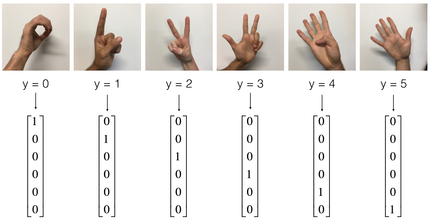
Figure 1: SIGNS dataset
Run the following code to load the dataset.
# Loading the dataset

X_train_orig, Y_train_orig, X_test_orig, Y_test_orig, classes = load_dataset()
Change the index below and run the cell to visualize some examples in the dataset.
# Example of a picture

index = 0

plt.imshow(X_train_orig[index])

print ("y = " + str(np.squeeze(Y_train_orig[:, index])))
y = 4

像往常那样flatten图像数据,并且用 x /= 255. 正则化数据。除此之外,你需要转换每个数字标签,为一个 one-hot向量,如 Figure 1.
# Flatten the training and test images

X_train_flatten = X_train_orig.reshape(X_train_orig.shape[0], -1).T

X_test_flatten = X_test_orig.reshape(X_test_orig.shape[0], -1).T

# Normalize image vectors

X_train = X_train_flatten/255.

X_test = X_test_flatten/255.

# Convert training and test labels to one hot matrices

Y_train = convert_to_one_hot(Y_train_orig, 6)

Y_test = convert_to_one_hot(Y_test_orig, 6)

print ("number of training examples = " + str(X_train.shape[1]))

print ("number of test examples = " + str(X_test.shape[1]))

print ("X_train shape: " + str(X_train.shape))

print ("Y_train shape: " + str(Y_train.shape))

print ("X_test shape: " + str(X_test.shape))

print ("Y_test shape: " + str(Y_test.shape))
number of training examples = 1080
number of test examples = 120
X_train shape: (12288, 1080)
Y_train shape: (6, 1080)
X_test shape: (12288, 120)
Y_test shape: (6, 120)
Note that 12288 comes from \(64 \times 64 \times 3\). Each image is square, 64 by 64 pixels, and 3 is for the RGB colors. Please make sure all these shapes make sense to you before continuing.
Your goal is to build an algorithm capable of recognizing a sign with high accuracy. To do so, you are going to build a tensorflow model that is almost the same as one you have previously built in numpy for cat recognition (but now using a softmax output).
The model is LINEAR -> RELU -> LINEAR -> RELU -> LINEAR -> SOFTMAX. (要输出多个分类)
2.1 - Create placeholders
Your first task is to create placeholders for X and Y. This will allow you to later pass your training data in when you run your session.
Exercise: Implement the function below to create the placeholders in tensorflow.
# GRADED FUNCTION: create_placeholders

def create_placeholders(n_x, n_y):

    """

    Creates the placeholders for the tensorflow session.

    Arguments:

    n_x -- scalar, size of an image vector (num_px * num_px = 64 * 64 * 3 = 12288)

    n_y -- scalar, number of classes (from 0 to 5, so -> 6)

    Returns:

    X -- placeholder for the data input, of shape [n_x, None] and dtype "float"

    Y -- placeholder for the input labels, of shape [n_y, None] and dtype "float"

    Tips:

    - You will use None because it let's us be flexible on the number of examples you will for the placeholders.

      In fact, the number of examples during test/train is different.

    """

    ### START CODE HERE ### (approx. 2 lines)

    X = tf.placeholder(tf.float32, shape=[n_x, None], name='X')

    Y = tf.placeholder(tf.float32, shape=[n_y, None], name='Y')

    ### END CODE HERE ###

    return X, Y
X, Y = create_placeholders(12288, 6)

print ("X = " + str(X))

print ("Y = " + str(Y))
X = Tensor("X_1:0", shape=(12288, ?), dtype=float32)
Y = Tensor("Y:0", shape=(6, ?), dtype=float32)
2.2 - Initializing the parameters
initialize the parameters in tensorflow.
Exercise: 在TensorFlow中初始化参数. 用 Xavier Initialization 对 weights 并且用 Zero Initialization for biases. As an example, to help you, for W1 and b1 you could use:
W1 = tf.get_variable("W1", [25,12288], initializer = tf.contrib.layers.xavier_initializer(seed = 1))

b1 = tf.get_variable("b1", [25,1], initializer = tf.zeros_initializer())
Please use seed = 1 to make sure your results match ours.
# GRADED FUNCTION: initialize_parameters

def initialize_parameters():

    """

    Initializes parameters to build a neural network with tensorflow. The shapes are:

                        W1 : [25, 12288]

                        b1 : [25, 1]

                        W2 : [12, 25]

                        b2 : [12, 1]

                        W3 : [6, 12]

                        b3 : [6, 1]

    Returns:

    parameters -- a dictionary of tensors containing W1, b1, W2, b2, W3, b3

    """

    tf.set_random_seed(1)                   # so that your "random" numbers match ours

    ### START CODE HERE ### (approx. 6 lines of code)

    W1 = tf.get_variable("W1", [25, 12288], initializer=tf.contrib.layers.xavier_initializer(seed=1))

    b1 = tf.get_variable("b1", [25, 1], initializer=tf.zeros_initializer())

    W2 = tf.get_variable("W2", [12, 25], initializer=tf.contrib.layers.xavier_initializer(seed=1))

    b2 = tf.get_variable("b2", [12, 1], initializer=tf.zeros_initializer())

    W3 = tf.get_variable("W3", [6, 12], initializer=tf.contrib.layers.xavier_initializer(seed=1))

    b3 = tf.get_variable("b3", [6, 1], initializer=tf.zeros_initializer())

    ### END CODE HERE ###

    parameters = {"W1": W1,

                  "b1": b1,

                  "W2": W2,

                  "b2": b2,

                  "W3": W3,

                  "b3": b3}

    return parameters
tf.reset_default_graph()

with tf.Session() as sess:

    parameters = initialize_parameters()

    print("W1 = " + str(parameters["W1"]))

    print("b1 = " + str(parameters["b1"]))

    print("W2 = " + str(parameters["W2"]))

    print("b2 = " + str(parameters["b2"]))
W1 = <tf.Variable 'W1:0' shape=(25, 12288) dtype=float32_ref>
b1 = <tf.Variable 'b1:0' shape=(25, 1) dtype=float32_ref>
W2 = <tf.Variable 'W2:0' shape=(12, 25) dtype=float32_ref>
b2 = <tf.Variable 'b2:0' shape=(12, 1) dtype=float32_ref>
2.3 - Forward propagation in tensorflow
implement the forward propagation module in tensorflow. The function will take in a dictionary of parameters and it will complete the forward pass. The functions you will be using are:
tf.add(...,...)to do an additiontf.matmul(...,...)to do a matrix multiplication(矩阵乘法)tf.nn.relu(...)to apply the ReLU activation
Question: Implement the forward pass of the neural network. We commented for you the numpy equivalents so that you can compare the tensorflow implementation to numpy. It is important to note that the forward propagation stops at z3. The reason is that in tensorflow the last linear layer output is given as input to the function computing the loss. Therefore, you don't need a3!
# GRADED FUNCTION: forward_propagation

def forward_propagation(X, parameters):

    """

    Implements the forward propagation for the model: LINEAR -> RELU -> LINEAR -> RELU -> LINEAR -> SOFTMAX

    Arguments:

    X -- input dataset placeholder, of shape (input size, number of examples)

    parameters -- python dictionary containing your parameters "W1", "b1", "W2", "b2", "W3", "b3"

                  the shapes are given in initialize_parameters

    Returns:

    Z3 -- the output of the last LINEAR unit

    """

    # Retrieve the parameters from the dictionary "parameters"

    W1 = parameters['W1']

    b1 = parameters['b1']

    W2 = parameters['W2']

    b2 = parameters['b2']

    W3 = parameters['W3']

    b3 = parameters['b3']

    ### START CODE HERE ### (approx. 5 lines)              # Numpy Equivalents:

    Z1 = tf.add(tf.matmul(W1, X), b1)                      # Z1 = np.dot(W1, X) + b1

    A1 = tf.nn.relu(Z1)                                    # A1 = relu(Z1)

    Z2 = tf.add(tf.matmul(W2, A1), b2)                     # Z2 = np.dot(W2, a1) + b2

    A2 = tf.nn.relu(Z2)                                    # A2 = relu(Z2)

    Z3 = tf.add(tf.matmul(W3, A2), b3)                     # Z3 = np.dot(W3,Z2) + b3

    ### END CODE HERE ###

    return Z3
tf.reset_default_graph()

with tf.Session() as sess:

    X, Y = create_placeholders(12288, 6)

    parameters = initialize_parameters()

    Z3 = forward_propagation(X, parameters)

    print("Z3 = " + str(Z3))
2.4 - Compute cost
As seen before, it is very easy to compute the cost using:
tf.reduce_mean(tf.nn.softmax_cross_entropy_with_logits(logits = ..., labels = ...))
Question: Implement the cost function below.
- It is important to know that the "
logits" and "labels" inputs oftf.nn.softmax_cross_entropy_with_logitsare expected to be of shape (number of examples, num_classes). We have thus transposed Z3 and Y for you. - Besides,
tf.reduce_meanbasically does the summation over the examples.
# GRADED FUNCTION: compute_cost

def compute_cost(Z3, Y):

    """

    Computes the cost

    Arguments:

    Z3 -- output of forward propagation (output of the last LINEAR unit), of shape (6, number of examples)

    Y -- "true" labels vector placeholder, same shape as Z3

    Returns:

    cost - Tensor of the cost function

    """

    # to fit the tensorflow requirement for tf.nn.softmax_cross_entropy_with_logits(...,...)

    logits = tf.transpose(Z3)   # 转置

    labels = tf.transpose(Y)

    ### START CODE HERE ### (1 line of code)

    # tf.reduce_mean 函数用于计算张量tensor沿着指定的数轴(tensor的某一维度)上的的平均值,

    # 主要用作降维或者计算tensor(图像)的平均值。

    cost = tf.reduce_mean(tf.nn.softmax_cross_entropy_with_logits(logits=logits,

                                                                 labels=labels))

    ### END CODE HERE ###

    return cost
tf.reset_default_graph()

with tf.Session() as sess:

    X, Y = create_placeholders(12288, 6)

    parameters = initialize_parameters()

    Z3 = forward_propagation(X, parameters)

    cost = compute_cost(Z3, Y)

    print("cost = " + str(cost))
cost = Tensor("Mean:0", shape=(), dtype=float32)
2.5 - Backward propagation & parameter updates
All the backpropagation and the parameters update is taken care of in 1 line of code.
After you compute the cost function. You will create an "optimizer" object. 选择优化函数(optimization) 和 learning rate 最小化代价。
For instance, for gradient descent the optimizer would be:
optimizer = tf.train.GradientDescentOptimizer(learning_rate = learning_rate).minimize(cost)
To make the optimization you would do:
_ , c = sess.run([optimizer, cost], feed_dict={X: minibatch_X, Y: minibatch_Y})
This computes the backpropagation by passing through the tensorflow graph in the reverse order. From cost to inputs.
Note When coding, we often use _ as a "throwaway" variable to store values that we won't need to use later. Here, _ takes on the evaluated value of optimizer, which we don't need (and c takes the value of the cost variable).
2.6 - Building the model
Now, you will bring it all together!
Exercise: Implement the model. You will be calling the functions you had previously implemented.
def model(X_train, Y_train, X_test, Y_test, learning_rate = 0.0001,

          num_epochs = 1500, minibatch_size = 32, print_cost = True):

    """

    Implements a three-layer tensorflow neural network: LINEAR->RELU->LINEAR->RELU->LINEAR->SOFTMAX.

    Arguments:

    X_train -- training set, of shape (input size = 12288, number of training examples = 1080)

    Y_train -- test set, of shape (output size = 6, number of training examples = 1080)

    X_test -- training set, of shape (input size = 12288, number of training examples = 120)

    Y_test -- test set, of shape (output size = 6, number of test examples = 120)

    learning_rate -- learning rate of the optimization

    num_epochs -- number of epochs of the optimization loop

    minibatch_size -- size of a minibatch

    print_cost -- True to print the cost every 100 epochs

    Returns:

    parameters -- parameters learnt by the model. They can then be used to predict.

    """

    ops.reset_default_graph()                         # to be able to rerun the model without overwriting tf variables

    tf.set_random_seed(1)                             # to keep consistent results

    seed = 3                                          # to keep consistent results

    (n_x, m) = X_train.shape                          # (n_x: input size, m : number of examples in the train set)

    n_y = Y_train.shape[0]                            # n_y : output size

    costs = []                                        # To keep track of the cost

    # Create Placeholders of shape (n_x, n_y)

    ### START CODE HERE ### (1 line)

    X, Y = create_placeholders(n_x, n_y)

    ### END CODE HERE ###

    # Initialize parameters

    ### START CODE HERE ### (1 line)

    parameters = initialize_parameters()

    ### END CODE HERE ###

    # Forward propagation: Build the forward propagation in the tensorflow graph

    ### START CODE HERE ### (1 line)

    Z3 = forward_propagation(X, parameters)

    ### END CODE HERE ###

    # Cost function: Add cost function to tensorflow graph

    ### START CODE HERE ### (1 line)

    cost = compute_cost(Z3, Y)

    ### END CODE HERE ###

    # Backpropagation: Define the tensorflow optimizer. Use an AdamOptimizer.

    ### START CODE HERE ### (1 line)

    optimizer = tf.train.AdamOptimizer(learning_rate=learning_rate).minimize(cost)

    ### END CODE HERE ###

    # Initialize all the variables

    init = tf.global_variables_initializer()

    # Start the session to compute the tensorflow graph

    with tf.Session() as sess:

        # Run the initialization

        sess.run(init)

        # Do the training loop

        for epoch in range(num_epochs):

            epoch_cost = 0.                       # Defines a cost related to an epoch

            num_minibatches = int(m / minibatch_size) # number of minibatches of size minibatch_size in the train set

            seed = seed + 1

            minibatches = random_mini_batches(X_train, Y_train, minibatch_size, seed)

            for minibatch in minibatches:

                # Select a minibatch

                (minibatch_X, minibatch_Y) = minibatch

                # IMPORTANT: The line that runs the graph on a minibatch.

                # Run the session to execute the "optimizer" and the "cost", the feedict should contain a minibatch for (X,Y).

                ### START CODE HERE ### (1 line)

                _, minibatch_cost = sess.run([optimizer, cost],

                                             feed_dict={X: minibatch_X,

                                                        Y: minibatch_Y})

                ### END CODE HERE ###

                epoch_cost += minibatch_cost / num_minibatches

            # Print the cost every epoch

            if print_cost == True and epoch % 100 == 0:

                print ("Cost after epoch %i: %f" % (epoch, epoch_cost))

            if print_cost == True and epoch % 5 == 0:

                costs.append(epoch_cost)

        # plot the cost

        plt.plot(np.squeeze(costs))

        plt.ylabel('cost')

        plt.xlabel('iterations (per tens)')

        plt.title("Learning rate =" + str(learning_rate))

        plt.show()

        # lets save the parameters in a variable

        parameters = sess.run(parameters)

        print ("Parameters have been trained!")

        # Calculate the correct predictions

        correct_prediction = tf.equal(tf.argmax(Z3), tf.argmax(Y))

        # Calculate accuracy on the test set

        accuracy = tf.reduce_mean(tf.cast(correct_prediction, "float"))

        print ("Train Accuracy:", accuracy.eval({X: X_train, Y: Y_train}))

        print ("Test Accuracy:", accuracy.eval({X: X_test, Y: Y_test}))

        return parameters
parameters = model(X_train, Y_train, X_test, Y_test)
Cost after epoch 0: 1.855702
Cost after epoch 100: 1.016458
Cost after epoch 200: 0.733102
Cost after epoch 300: 0.572939
Cost after epoch 400: 0.468774
Cost after epoch 500: 0.381021
Cost after epoch 600: 0.313827
Cost after epoch 700: 0.254280
Cost after epoch 800: 0.203799
Cost after epoch 900: 0.166512
Cost after epoch 1000: 0.140937
Cost after epoch 1100: 0.107750
Cost after epoch 1200: 0.086299
Cost after epoch 1300: 0.060949
Cost after epoch 1400: 0.050934
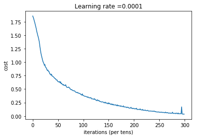
Parameters have been trained!
Train Accuracy: 0.999074
Test Accuracy: 0.725
2.7 - Test with your own image
# import scipy

# from PIL import Image

# from scipy import ndimage

import imageio

from skimage.transform import resize

## START CODE HERE ## (PUT YOUR IMAGE NAME)

my_image = "thumbs_up.jpg"

## END CODE HERE ##

# We preprocess your image to fit your algorithm.

fname = "images/" + my_image

# image = np.array(ndimage.imread(fname, flatten=False))

# my_image = scipy.misc.imresize(image, size=(64,64)).reshape((1, 64*64*3)).T

image = np.array(imageio.imread(fname))                   # 读入图片为矩阵, 这里用原版本的会出错,scipy的那个函数被删了

# print(image.shape)

# 转置图片为 (num_px*num_px*3, 1)向量

my_image = resize(image, output_shape=(64, 64)).reshape((1, 64 * 64 * 3)).T

# print(my_image)

my_image_prediction = predict(my_image, parameters)

plt.imshow(image)

print("Your algorithm predicts: y = " + str(np.squeeze(my_image_prediction)))
最新文章
- pythonchallenge 解谜
- 【代码笔记】iOS-检测手机翻转
- Spring整合Hibernate。。。。
- (转载)loadrunner简单使用——HTTP,WebService,Socket压力测试脚本编写
- Difference between datacontract and messagecontract in wcf
- 【iOS发展-81】setNeedsDisplay刷新显卡,并CADisplayLink它用来模拟计时器效果
- canvas常用api
- 曾经进公司面试的C语言有关指针和数组的笔试题
- 显著性检测(saliency detection)评价指标之sAUC(shuffled AUC)的Matlab代码实现
- android 下改变默认的checkbox的 选中 和被选中 图片
- (转) How a Kalman filter works, in pictures
- js的回调函数详解
- requestAnimationFrame 完美兼容封装
- IDEA项目搭建三——简单配置Maven使用国内及本地仓库
- md5目录下的文件包括子目录
- 使用tensorflow-serving部署tensorflow模型
- JS时间戳转时间格式
- 【日常训练】Help Victoria the Wise(Codeforces 99C)
- [!] Attempt to read non existent folder `***********`
- (二)Linux Shell编程——运算符、注释