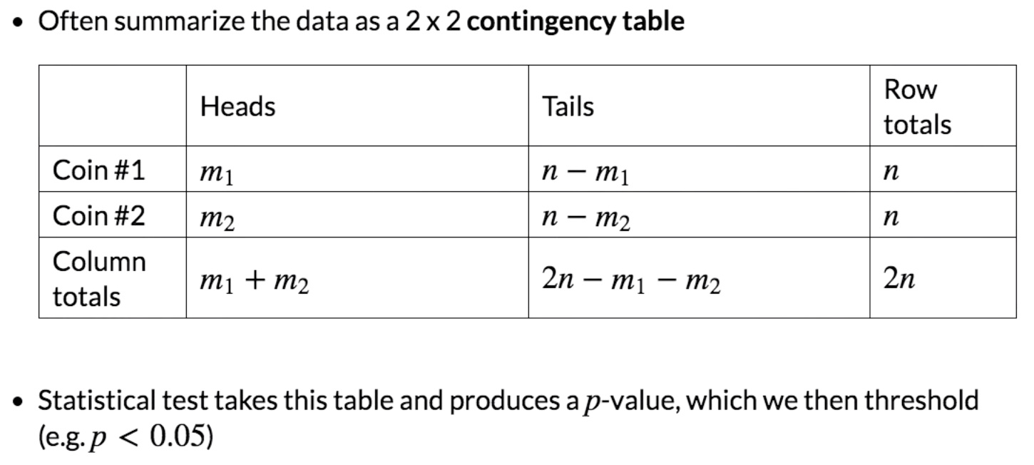
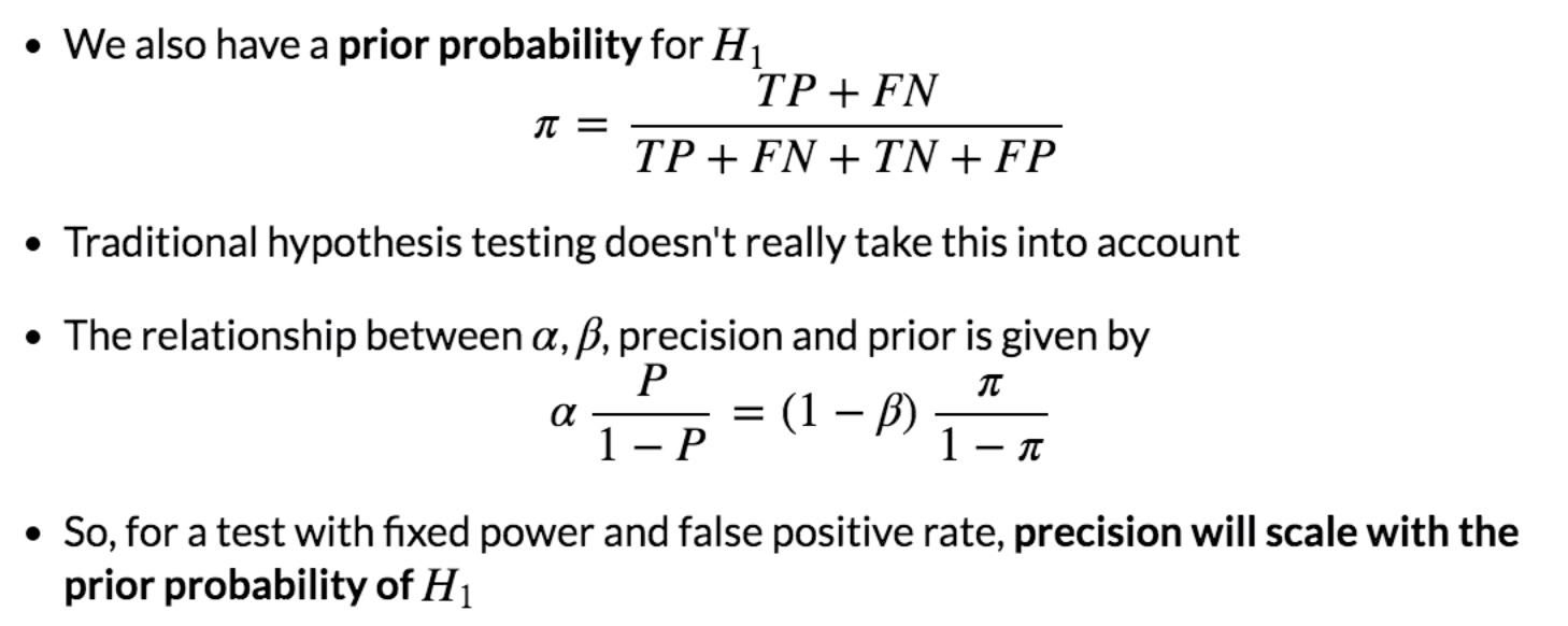
A/B Testing with Practice in Python (Part One)
I learned A/B testing from a Youtube vedio. The link is https://www.youtube.com/watch?v=Bu7OqjYk0jM.
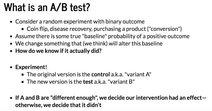
I will divide the note into two parts. The first part is generally an overview of hypothesis testing. Most concepts can be found in the article "Statistics Basics: Main Concepts in Hypothesis Testing" and I will focus on pratical applications here.
|
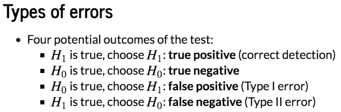
Actual Predicted |
T (H1) | F (H0) |
| T (H1) | TP | FP (α) |
| F (H0) | FN (β) | TN |
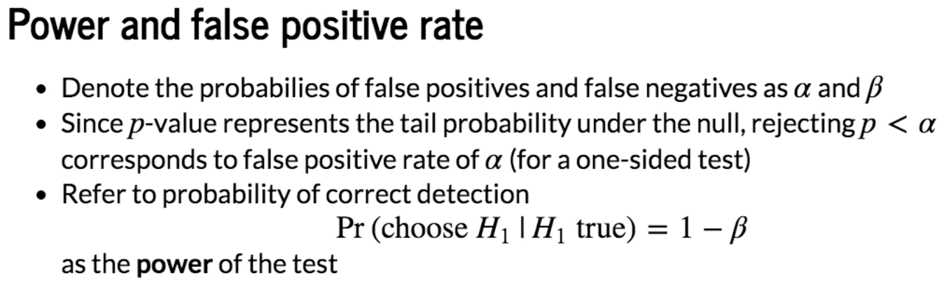
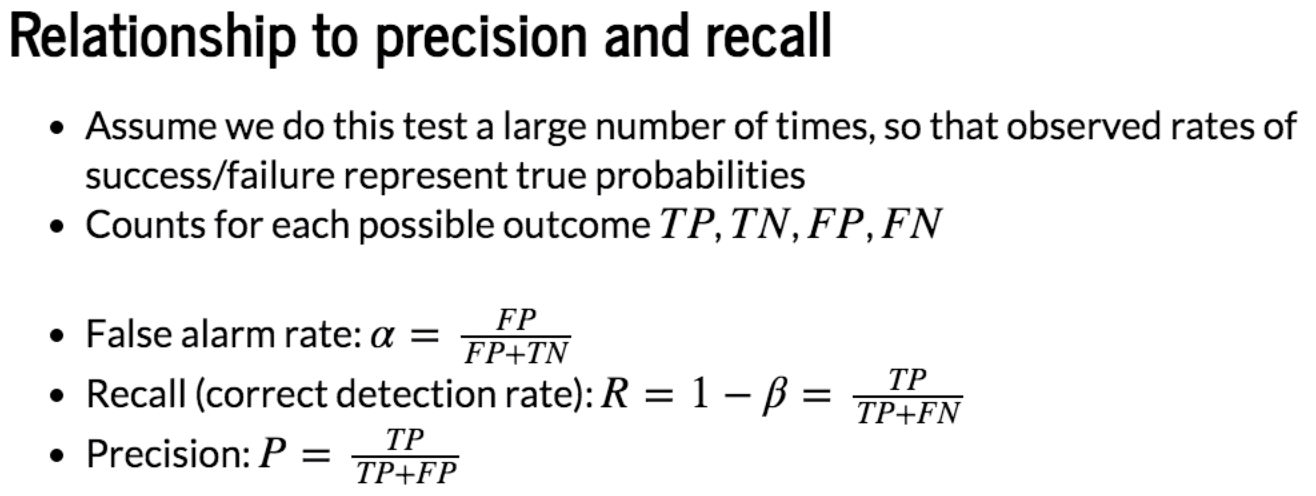
P = TP/(TP+FN)
R = 1-β =TP/(TP+FN)
Python Example
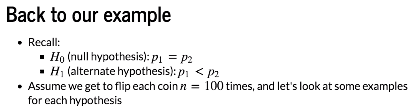
Case #1: Alternate hypothesis is true
n = 100

p1 = 0.4

p2 = 0.6

# Compute distributions

x = np.arange(0,n+1)

pmf1 = stats.binom.pmf(x,n,p1)

pmf2 = stats.binom.pmf(x,n,p2)

plot(x,pmf1,pmf2)
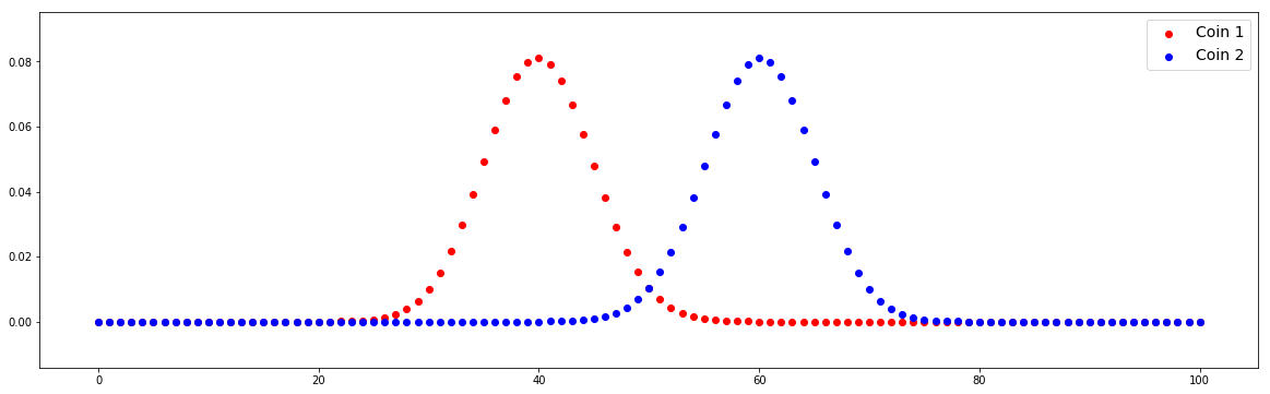
We can find that the distributions between Coin 1 and Coin 2 are different. We check different values of m1 and m2.
# Example outcomes

m1, m2 = 40, 60

table = [[m1, n-m1], [m2, n-m2]]

chi2, pval, dof, expected = stats.chi2_contingency(table)

decision = 'reject H0' if pval<0.05 else 'accept H0'

print('{} ({})'.format(pval,decision))
0.007209570764742524 (reject H0)
# Example outcomes

m1, m2 = 43, 57

table = [[m1, n-m1], [m2, n-m2]]

chi2, pval, dof, expected = stats.chi2_contingency(table)

decision = 'reject H0' if pval<0.05 else 'accept H0'

print('{} ({})'.format(pval,decision))
0.06599205505934735 (accept H0)
In the secod example, m1 and m2 are not different significantly to reject H0.
Case #2: Null hypothesis is true
n = 100

p1 = 0.5

p2 = 0.5

# Compute distributions

x = np.arange(0,n+1)

pmf1 = stats.binom.pmf(x,n,p1)

pmf2 = stats.binom.pmf(x,n,p2)

plot(x,pmf1,pmf2)
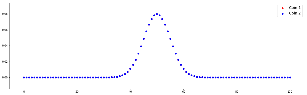
In this case, two distributions overlap because we define the same value of p1 and p2.
# Example outcomes

m1, m2 = 49, 51

table = [[m1, n-m1], [m2, n-m2]]

chi2, pval, dof, expected = stats.chi2_contingency(table)

decision = 'reject H0' if pval<0.05 else 'accept H0'

print('{} ({})'.format(pval,decision))
0.887537083981715 (accept H0)
Actuall, we can only say that m1 and m2 are not different significantly to reject H0. It doesn't mean we should accept H0. The explanation is given in the previous article.
# Example outcomes

m1, m2 = 42, 58

table = [[m1, n-m1], [m2, n-m2]]

chi2, pval, dof, expected = stats.chi2_contingency(table)

decision = 'reject H0' if pval<0.05 else 'accept H0'

print('{} ({})'.format(pval,decision))
0.033894853524689295 (reject H0)


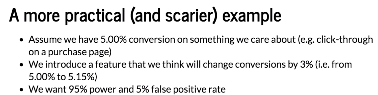
Firstly, calculate the sample size:
p1, p2 = 0.0500, 0.0515

alpha = 0.05

beta = 0.05

# Evaluate quantile function

p_bar = (p1+p2)/2.0

za = stats.norm.ppf(1-alpha/2) # Two-sided test

zb = stats.norm.ppf(1-beta)

# Compute correction factor

A = (za*np.sqrt(2*p_bar*(1-p_bar))+ zb*np.sqrt(p1*(1-p1)+p2*(1-p2)))**2

#Estimate samples required

n = A*(((1+np.sqrt(1+4*(p1-p2)/A)))/(2*(p1-p2)))**2

print (n) # we need 2n users
555118.7638311392
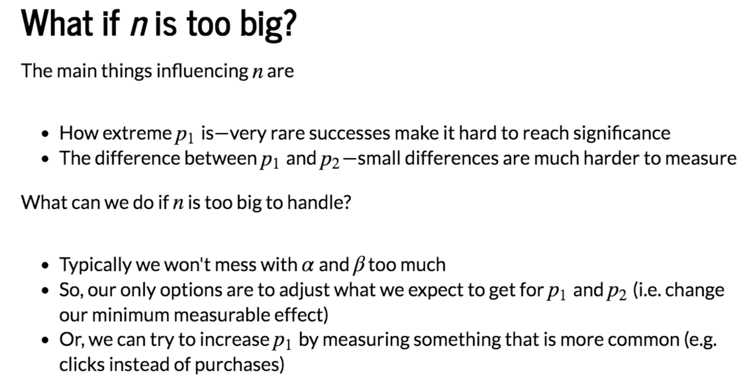
So for test and control combined we'll need at least 2n = 1.1 million users. This is where this stuff gets hard and you're trying to measure something that doesn't happen often which is usally the thing to care because if it's rare, it's usually valuable. When you're trying to change it, you usually can't change it much because if you can change it a lot then your business would be easier usually it's harder to change the thing you care the most about. So in that case, it's like the hardest case where a/b testing the most values are unchange.
Next we can perform a/b testing:
n = 555119

n_trials = 10000

# Simulate experimental results when null is true

control0 = stats.binom.rvs (n,p1,size = n_trials)

test0 = stats.binom.rvs(n, p1, size = n_trials) # Test and control are the same

tables0 = [[[a, n-a], [b, n-b]] for a, b in zip(control0, test0)]

results0 = [stats.chi2_contingency(T) for T in tables0]

decisions0 = [x[1] <= alpha for x in results0]

# Simulate experimental results when alternate is true

control1 = stats.binom.rvs (n,p1,size = n_trials)

test1 = stats.binom.rvs(n, p2, size = n_trials) # Test and control are the same

tables1 = [[[a, n-a], [b, n-b]] for a, b in zip(control1, test1)]

results1 = [stats.chi2_contingency(T) for T in tables1]

decisions1 = [x[1] <= alpha for x in results1]

# Compute false alarm and correct detection rates

alpha_est = sum(decisions0)/float(n_trials)

power_est = sum(decisions1)/float(n_trials)

print('Theoretical false alarm rate = {:0.4f}, '.format(alpha)+

     'empirical false alarm rate = {:0.4f}'.format(alpha_est))

print('Theoretical power = {:0.4f}, '.format(1-beta)+

     'empirical power = {:0.4f}'.format(power_est))
Theoretical false alarm rate = 0.0500, empirical false alarm rate = 0.0509

Theoretical power = 0.9500, empirical power = 0.9536
最新文章
- Linux常用获取进程占用资源情况手段
- RabbitMQ 集群
- android Gui系统之SurfaceFlinger(2)---BufferQueue
- ubuntu14.04 server 安装vmware worktation 12
- 参数(parameter)和属性(Attribute)的区别
- 解决stackoverflow打开慢不能注册登录
- mybatis 3.2.3 maven dependency pom.xml 配置
- quick -- 添加按钮
- PHP人民币金额数字转中文大写的函数
- JAVA基础-子类继承父类实例化对象过程
- VB,VBS,VBA,ASP可引用的库参考
- java学习笔记 --- java基础语法
- Python实战之文件操作的详细简单练习
- 移动端300ms点击延迟
- C++的反思[转]
- 虚拟机中安装Ubuntu后,安装VMwareTools出错的解决办法:Not enough free space to extract VMwareTools
- quartz 2.1.6使用方法
- 小程序之取标签中内容 例如view,text
- 【轻松前端之旅】元素,标记,属性,<html>标签
- 微信Tinker的一切都在这里,包括源码(一)