《DSP using MATLAB》Problem 8.32
2024-10-07 22:03:31
代码:
%% ------------------------------------------------------------------------
%% Output Info about this m-file
fprintf('\n***********************************************************\n');
fprintf(' <DSP using MATLAB> Problem 8.32 \n\n'); banner();
%% ------------------------------------------------------------------------ % -------------------------------------
% Ω=(2/T)tan(ω/2)
% ω=2*[atan(ΩT/2)]
% Digital Filter Specifications:
% -------------------------------------
wp = 0.3*pi; % digital passband freq in rad
ws = 0.4*pi; % digital stopband freq in rad
Rp = 0.25; % passband ripple in dB
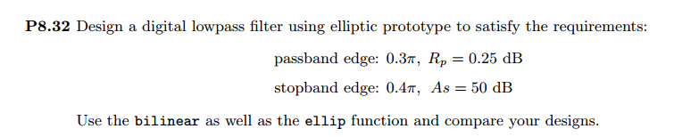
As = 50; % stopband attenuation in dB Ripple = 10 ^ (-Rp/20) % passband ripple in absolute
Attn = 10 ^ (-As/20) % stopband attenuation in absolute % Analog prototype specifications: Inverse Mapping for frequencies
T = 1; % set T = 1
Fs = 1/T;
OmegaP = (2/T)*tan(wp/2) % prototype passband freq
OmegaS = (2/T)*tan(ws/2) % prototype stopband freq % Analog Elliptic Prototype Filter Calculation:
[cs, ds] = afd_elip(OmegaP, OmegaS, Rp, As); % Calculation of second-order sections:
fprintf('\n***** Cascade-form in s-plane: START *****\n');
[CS, BS, AS] = sdir2cas(cs, ds)
fprintf('\n***** Cascade-form in s-plane: END *****\n'); % Calculation of Frequency Response:
[db_s, mag_s, pha_s, ww_s] = freqs_m(cs, ds, 0.5*pi/T); % Calculation of Impulse Response:
[ha, x, t] = impulse(cs, ds); % Impulse Invariance Transformation:
%[b, a] = imp_invr(cs, ds, T); % Bilinear Transformation
[b, a] = bilinear(cs, ds, Fs)
[C, B, A] = dir2cas(b, a) % Calculation of Frequency Response:
[db, mag, pha, grd, ww] = freqz_m(b, a); %% -----------------------------------------------------------------
%% Plot
%% -----------------------------------------------------------------
figure('NumberTitle', 'off', 'Name', 'Problem 8.32 Analog Elliptic lowpass')
set(gcf,'Color','white');
M = 1.0; % Omega max subplot(2,2,1); plot(ww_s/pi, mag_s); grid on; %axis([-10, 10, 0, 1.2]);
xlabel(' Analog frequency in \pi units'); ylabel('|H|'); title('Magnitude in Absolute');
set(gca, 'XTickMode', 'manual', 'XTick', [-0.4625, -0.3244, 0, 0.3244, 0.4625]);
set(gca, 'YTickMode', 'manual', 'YTick', [0, 0.0032, 0.9716, 1.0, 1.5]); subplot(2,2,2); plot(ww_s/pi, db_s); grid on; %axis([0, M, -50, 10]);
xlabel('Analog frequency in \pi units'); ylabel('Decibels'); title('Magnitude in dB ');
set(gca, 'XTickMode', 'manual', 'XTick', [-0.4625, -0.3244, 0, 0.3244, 0.417, 0.458, 0.4625]);
set(gca, 'YTickMode', 'manual', 'YTick', [-50, -1, 0]);
set(gca,'YTickLabelMode','manual','YTickLabel',['50';' 1';' 0']); subplot(2,2,3); plot(ww_s/pi, pha_s/pi); grid on; %axis([-10, 10, -1.2, 1.2]);
xlabel('Analog frequency in \pi nuits'); ylabel('radians'); title('Phase Response');
set(gca, 'XTickMode', 'manual', 'XTick', [-0.4625, -0.3244, 0, 0.3244, 0.4625]);
set(gca, 'YTickMode', 'manual', 'YTick', [-1:0.5:1]); subplot(2,2,4); plot(t, ha); grid on; %axis([0, 30, -0.05, 0.25]);
xlabel('time in seconds'); ylabel('ha(t)'); title('Impulse Response'); figure('NumberTitle', 'off', 'Name', 'Problem 8.32 Digital Elliptic lowpass by bilinear')
set(gcf,'Color','white');
M = 2; % Omega max subplot(2,2,1); plot(ww/pi, mag); axis([0, M, 0, 1.2]); grid on;
xlabel(' Digital frequency in \pi units'); ylabel('|H|'); title('Magnitude Response');
set(gca, 'XTickMode', 'manual', 'XTick', [0, 0.3, 0.4, 1.6, 1.7, M]);
set(gca, 'YTickMode', 'manual', 'YTick', [0, 0.0032, 0.9716, 1]); subplot(2,2,2); plot(ww/pi, pha/pi); axis([0, M, -1.1, 1.1]); grid on;
xlabel('Digital frequency in \pi nuits'); ylabel('radians in \pi units'); title('Phase Response');
set(gca, 'XTickMode', 'manual', 'XTick', [0, 0.3, 0.4, 1.6, 1.7, M]);
set(gca, 'YTickMode', 'manual', 'YTick', [-1:1:1]); subplot(2,2,3); plot(ww/pi, db); axis([0, M, -80, 10]); grid on;
xlabel('Digital frequency in \pi units'); ylabel('Decibels'); title('Magnitude in dB ');
set(gca, 'XTickMode', 'manual', 'XTick', [0, 0.3, 0.37, 0.4, 1.6, 1.7, M]);
set(gca, 'YTickMode', 'manual', 'YTick', [-60, -50, -1, 0]);
set(gca,'YTickLabelMode','manual','YTickLabel',['60';'50';' 1';' 0']); subplot(2,2,4); plot(ww/pi, grd); grid on; %axis([0, M, 0, 35]);
xlabel('Digital frequency in \pi units'); ylabel('Samples'); title('Group Delay');
set(gca, 'XTickMode', 'manual', 'XTick', [0, 0.3, 0.4, 1.6, 1.7, M]);
%set(gca, 'YTickMode', 'manual', 'YTick', [0:5:35]); figure('NumberTitle', 'off', 'Name', 'Problem 8.32 Pole-Zero Plot')
set(gcf,'Color','white');
zplane(b,a);
title(sprintf('Pole-Zero Plot'));
%pzplotz(b,a); % ----------------------------------------------
% Calculation of Impulse Response
% ----------------------------------------------
figure('NumberTitle', 'off', 'Name', 'Problem 8.32 Imp & Freq Response')
set(gcf,'Color','white');
t = [0:0.01:90]; subplot(2,1,1); impulse(cs,ds,t); grid on; % Impulse response of the analog filter
axis([0,90,-0.2,0.3]);hold on n = [0:1:90/T]; hn = filter(b,a,impseq(0,0,90/T)); % Impulse response of the digital filter
stem(n*T,hn); xlabel('time in sec'); title (sprintf('Impulse Responses T=%2d',T));
hold off % Calculation of Frequency Response:
[dbs, mags, phas, wws] = freqs_m(cs, ds, 2*pi/T); % Analog frequency s-domain [dbz, magz, phaz, grdz, wwz] = freqz_m(b, a); % Digital z-domain %% -----------------------------------------------------------------
%% Plot
%% ----------------------------------------------------------------- subplot(2,1,2); plot(wws/(2*pi), mags/T,'b', wwz/(2*pi*T), magz, 'r'); grid on; xlabel('frequency in Hz'); title('Magnitude Responses'); ylabel('Magnitude'); text(-0.8,0.15,'Analog filter', 'Color', 'b'); text(0.8,0.4,'Digital filter', 'Color', 'r');
运行结果:
这里主要放双线性变化法的代码。
通带、阻带绝对指标,模拟滤波器截止频率指标,
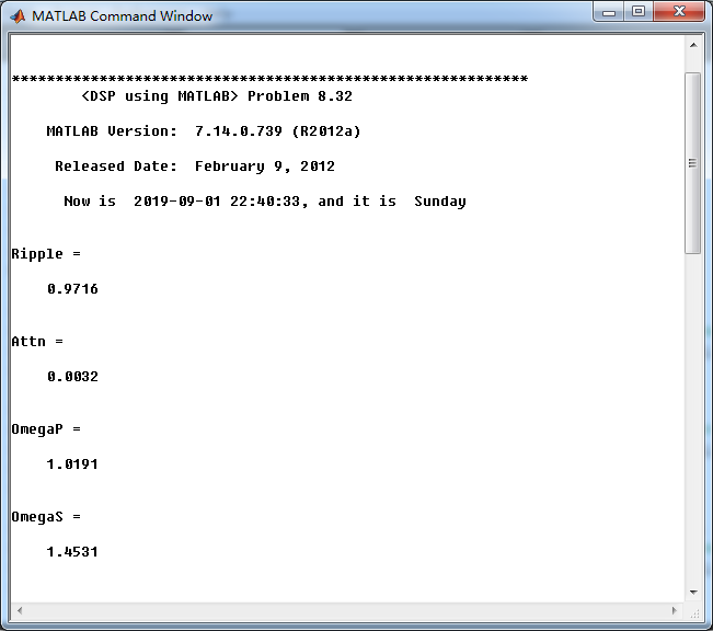
模拟Elliptic原型低通滤波器,系统函数串联形式的系数
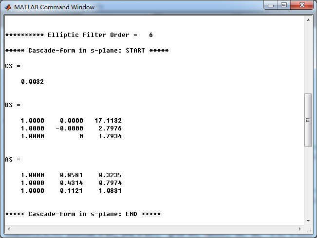
采用双线性变换法,得到数字Elliptic低通滤波器,系统函数直接形式的系数,转换成串联形式的系数
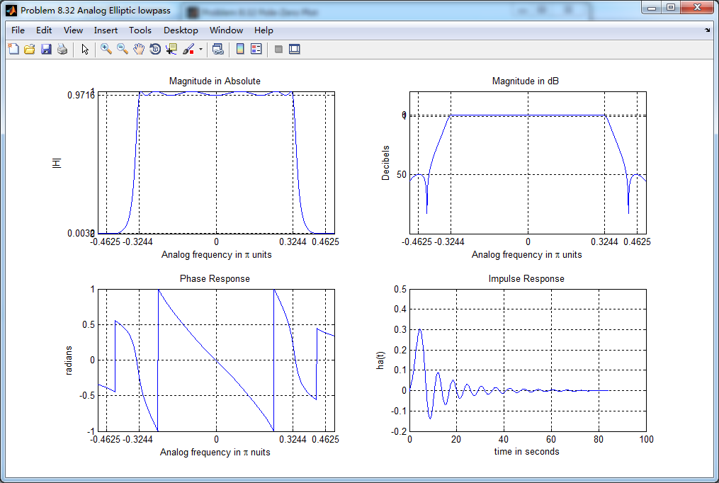
模拟Elliptic原型低通滤波器,其幅度谱、相位谱和脉冲响应
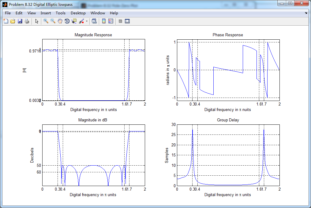
采用双线性变换法(bilinear)得到数字Elliptic低通滤波器,其幅度谱、相位谱和群延迟响应
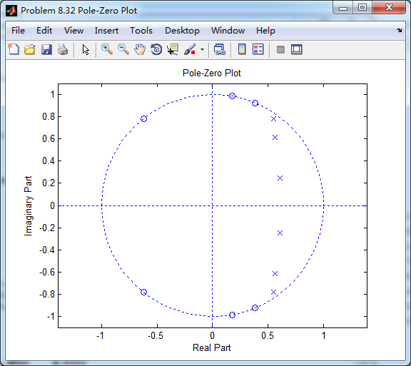
数字Elliptic低通系统函数零极点图
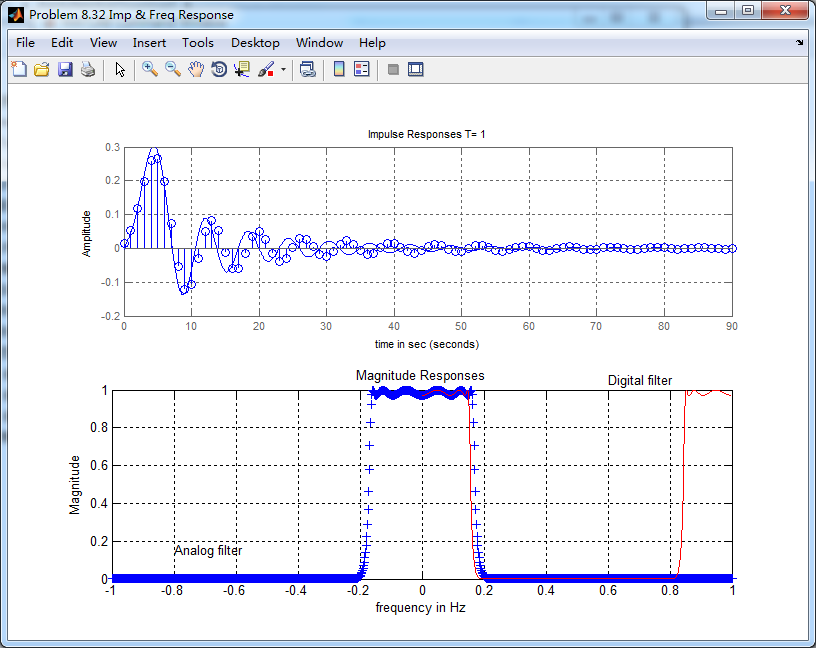
模拟原型和数字低通的脉冲响应对比,可见双线性变换法不保留脉冲响应的形态。
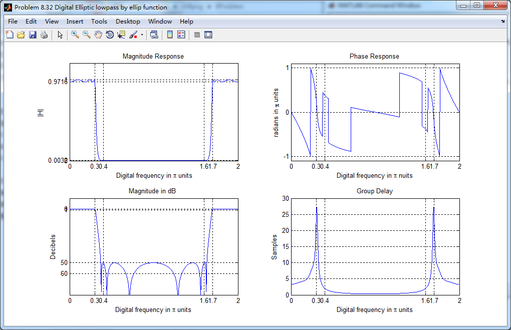
使用MATLAB自带ellip函数的运算结果这里就不写了,只放张幅度谱、相位谱和群延迟响应的图,可见和双线性变换法得到的结果相比,区别不大。
最新文章
- 5G关键技术评述
- STM32F103之DMA
- 使用AutoIT对增加和删除文件属性的实现
- 面向对象to1
- SharePoint Online 创建门户网站系列之准备篇
- Linux下防火墙开启相关端口及查看已开启端口
- C#分层开发MySchool
- 调试带有源代码的DLL文件
- Windows XP硬盘安装Ubuntu 12.04双系统图文详解
- simplePagination API
- [LeetCode] 032. Longest Valid Parentheses (Hard) (C++)
- dom4j解析xml文档全面介绍
- netty使用从0到1
- Java进阶(三十五)java int与integer的区别
- jquery-confirm使用方法
- Hbase思维导图之调优
- ajax readystatue
- Struts与jsp+javabean+servlet区别
- Nginx 介绍
- wireshark提取gzip格式的html